Abstract: The basic concept of the Wolfram Model is to determine rules for updating collection of relation. However, for a particular collection of relations and rules, there might be more than one way in which a given rule can be applied, creating the idea of multiway systems such as multiway string substitution systems. The aim of this project is to explore the multiway behaviors, such as connectivity of branchial structure, of one specific discrete model of computation: the Mobile Automaton. As multiway Turing Machines can be generated by combining multiple rules of ordinary Turing Machines, multiway Mobile Automata can also be created in this manner. Furthermore, another approach to the study of multiway systems taken in this project is the generation of multi-headed Mobile Automata, meaning that more than one active cells is being updated at each step, and the analysis of their multiway behavior as the intermediate case between the combined rules of single-headed Mobile Automata and multiway string substitution systems.
Multiway Mobile Automaton
Multiway Mobile Automaton
With the recent advancement of the Wolfram Physics Project, the study of multiway systems has being increasingly more relevant to the Wolfram Models and, more especially, to the study of quantum mechanics in the Wolfram framework. An example for which an ordinary system is transformed into a multiway system in order to study its general multiway features is the case of Multiway Turing Machines. There, different rules can be applied to the same configuration of the state being updated, which generates many possible paths of evolution for the system. For the mobile automaton case, a similar methodology will be applied in order to explore its multiway behaviors.
Review on Ordinary Mobile Automaton
Review on Ordinary Mobile Automaton
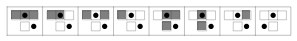
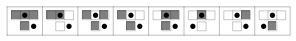
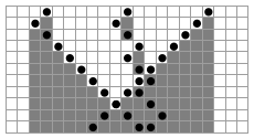
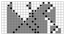
An ordinary mobile automaton is a similar case to cellular automata, with the exception that instead of having all the cells in the state being updated at the same time, only one active cells gets updated at a time according to a specific rule. The picture below shows 2 examples of mobile automata being updated for 10 steps, where the active cells is represented by the black dot and the rules used are shown below.
Out[]=
,
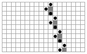
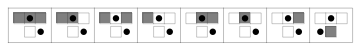
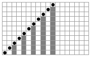
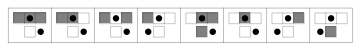
Throughout this project, the rules for the mobile automata will be specified as a list of two numbers, where the first number, as a binary list of 8 digits, represents the color (black or white) that the updated cell will turn after an update, and the second number, also as a binary list of 8 digits, represents the position (right or left) of the active cells after an update.
Introduction to Multiway Mobile Automaton
Introduction to Multiway Mobile Automaton
Combining 2 rules
Combining 2 rules
In a multiway mobile automaton, different rules are combined and more than one possible outcome can be specified for a particular case in the multiway system. An example of two individual rules being combined can be seen as
Out[]=
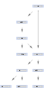
The result is that there can be many possible paths of evolution for the system—as represented by a multiway graph that connects successive possible configurations:
Out[]=
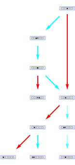
The evolution according to the ordinary mobile automaton rule corresponds to a particular path in the multiway graph, here represented by the different colors (colors are not representing only the evolution from the initial state, but also what rule is being applied to each state of the evolution):
Out[]=
|
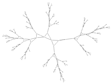
Running the systems for a few more steps, one can start to see more complex branching and merging patterns in the multiway system:
Out[]=
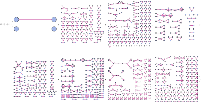
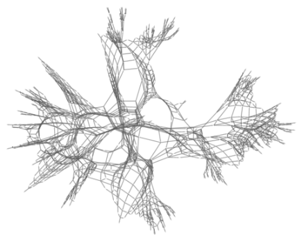
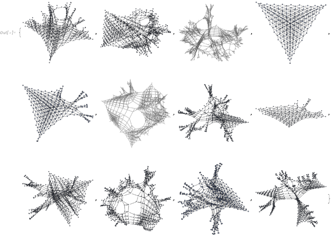
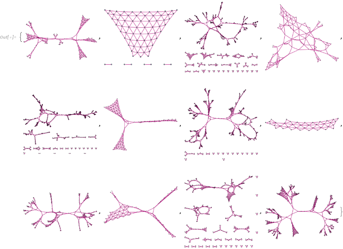
More examples of multiway mobile automata can be generated by combining randomly chosen rules:
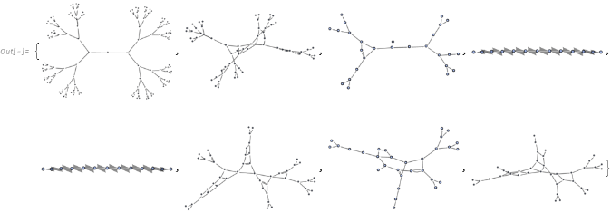
By looking at this graphs, one can see that one common patter for such multiway systems is the tree-like behavior of branching. In order to understand their multiway graphs in a more accurate way, one can use the structure of branchial graphs. Constructing the branchial graphs for the same chosen rules, we get:
Which confirms the expectation of tree-like systems with very disconnected branchial systems. One way that we can go around the disconnectivity of the branchial graphs is by implementing more rules for with a specific combination of cells in a state can be updated with.
Combining 4 rules
Combining 4 rules
Doing the same process for when 4 rules are combined and updating the states 6 times, we have states graph structures such as:
Now, in order to understand how connected the structure of the multiway system is, we again look at their branchial graphs:
As expected, more complex and connected structures are generated in their branchial structures. However, disconnectivity is still dominant, so an obvious next step is to implement more rules together so more possible paths could be achieved for a specific combination of cells in a state.
Combining 8 rules
Combining 8 rules
Again, repeating the same process of generating states graph structures after 6 steps:
And their branchial graphs:
Even though complexity and merging seems to emerge in the branchial graphs as we combine more and more rules, disconnectivity is still dominant in the overall structure, indicating that the multiway systems branches much like binomial trees. A reasonable estimation is that with a greater amount of rules combined, more connected branchial structures will emerge, but this amount would be extremely computationally expensive. For more connectivity in the multiway systems, however, another approach can be taken when dealing with multiway mobile automata, as described in the next section.
Multi-headed Mobile Automaton
Multi-headed Mobile Automaton
Ordinary Multi-headed Mobile Automaton
Ordinary Multi-headed Mobile Automaton
A second approach to explore multiway systems with mobile automata is to generate multi-headed automata, meaning that more than one cell can be updated at each step, which can be expected to generate more possibilities of connectivity for when the system is given rules that can generate multiple outputs given a collection of cells on a state. For visualisation purposes of the multi-headed mobile automaton, we give the following examples with initial states containing 2, 3 and 4 active cells:
Out[]=
,
,
Here the set of rules used are being used for each individual head on the initial state (first rule applies to first active cell, second rule applies to second active cell, and so on). As the different heads cross, they simply continue their specified paths according to their rules, not having any kind of interaction.
With that said, a multiway system can be generated using this new model of updating discrete model of computation.
Multiway Multi-headed Mobile Automaton
Multiway Multi-headed Mobile Automaton
3 active cells
3 active cells
With the multi-headed mobile automaton function, the multiway system generated with it seems to reproduce much more complex and connected states as the function is updated, since each rule can be applied to all the actives cells in a given state.
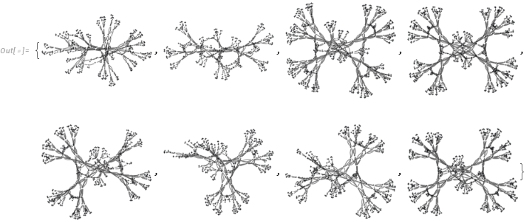
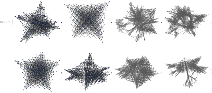
Starting with three heads in the initial state, the states graph structure already seem richer in connectivity and not as tree-like as with the case of the single-head multiway system:
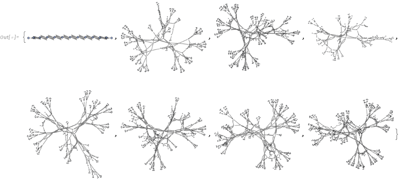
Generating randomly selected rules being applied to each head and random positions of the cells, we get a collection of states graphs after 10 steps of updates such as:
Their respective branchial graphs look much better:
5 active cells
5 active cells
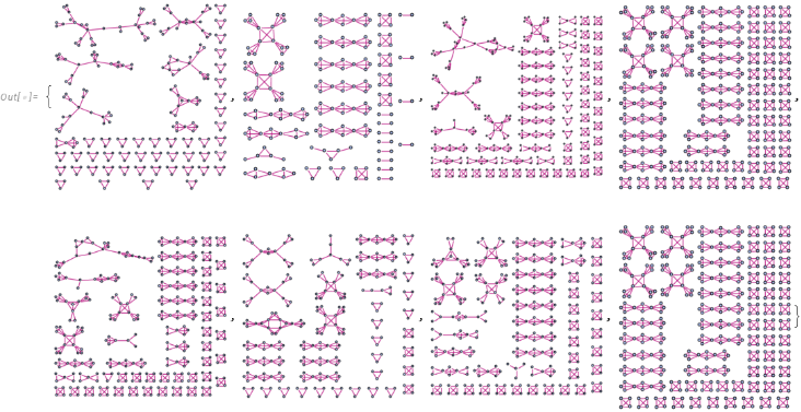
Conducting the same process for now 5 active cells on the initial tape and updating it for 7 steps, their states graph structure look like this:
And their respective branchial graphs being:
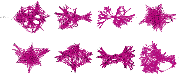
The trend of getting more complex and connected branchial graphs as we increase the number of heads in the initial tape is clearly observed. This leads the project to generate different metrics for calculating the complexity of the multiway structures, as described in the following section.
Branchial Complexity Metrics
Branchial Complexity Metrics
Instead of visually analyzing the connectivity of the branchial structures, connectivity metrics are applied to the different branchial graphs developed throughout the progress of the project, enabling a more accurate comparison between each step developed.
Graph Distance Matrix
Graph Distance Matrix
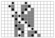
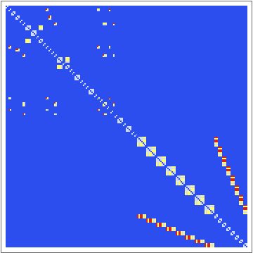
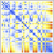
One way the branchial complexity of the multiway systems can be measured is by calculating the distance matrices of each branchial graph.
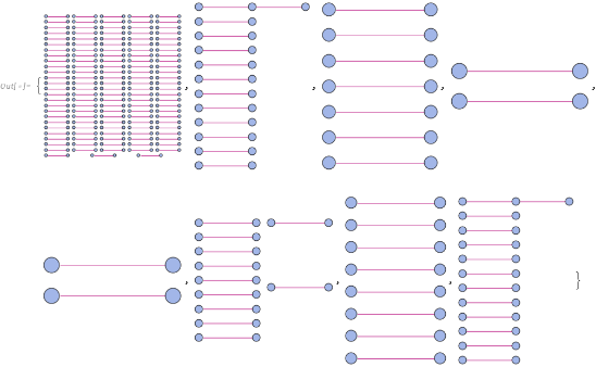
As an example, systems with 8 different rules combined for the evolution of a single-headed mobile automaton have distances matrix, after 6 steps, such as:
Out[]=
,
,
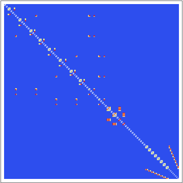
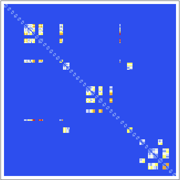
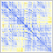
Now, applying the distance matrices function to the multi-headed automaton composed of 3 active cell and being updated for 10 steps, the graph distance matrices of their branchial graphs look like this:
Out[]=
,
,
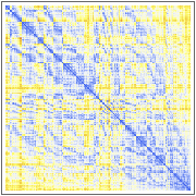
Much more complex structures can be seen on these matrices graphs, corresponding to a greater amount of merging and connectivity present in the branchial structures.
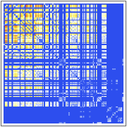
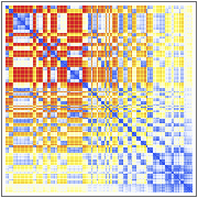
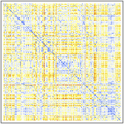
Applying the same operation for multi-headed automaton now composed of 5 active cells and being updated for 7 steps, the graph distance matrices are:
Out[]=
,
,
States Growth
States Growth
Another way for which the complexity of the branchial graphs can be measured is by calculating the amount of vertices the branchial structures have, called here as the states growth, and comparing it with the amount of vertices on branchial structures of systems with more active cells on the initial tapes. By looking at the branchial graphs as we increase the number of heads, a reasonable prediction would be to argue of an increasingly amount of vertices.
In order to achieve such a metric, the amount of vertices on branchial graphs is accomplished by averaging the number of vertices over a given amount of systems with randomly generated rules. Comparing the branchial graphs of the multi-headed automata system up to 7 active cells and updating them up to 8 steps, the number of vertices can be plotted such as:
In order to achieve such a metric, the amount of vertices on branchial graphs is accomplished by averaging the number of vertices over a given amount of systems with randomly generated rules. Comparing the branchial graphs of the multi-headed automata system up to 7 active cells and updating them up to 8 steps, the number of vertices can be plotted such as:
Out[]=
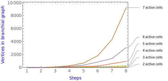
As expected, the greater the amount of active cells on the initial state of the multiway multi-headed automaton, the greater the number of vertices on their branchial graphs.
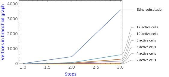
Also, another measurement that is worth taking is by applying the same process of counting vertices on branchial graphs as described above, but also considering a string substitution system where the initial tape has the same amount of characters as the amount of cells on the multi-headed automaton and the same amount of substitution can be applied to each character on the string as the amount of rules that can be applied to each cells on the state of the automaton . By doing that, the string substitution system can be thought of as a limit to the process of increasing the number of heads on the state of the system, since this process is simulating a state for which all the cells on it are active and multiple rules can be applied to each of them.
Out[]=
Concluding remarks
Concluding remarks
As this project proceeded, the single-headed mobile automaton did not show a great amount of complexity in their multiway structures. Even with more rules being put together, which consequently increases the possibilities of branching in the multiway systems, their branchial structures still showed predominant disconnectivity. With the second part of this project, however, multiway structures seemed to grow more and more complex with the implementation of the multi-headed mobile automaton. This new function showed a greater amount of merging in their branchial structures, which makes these new cases more compelling to the analyzes directed by the Wolfram Physics Project.
Following the trend of multicomputation research that has been produced, such as the work onMultiway Turing Machines and n-machines, some possible further steps on this project could be achieved by implementing causal structures on multiway mobile automaton and also its applications as models of computation can be used to probe physical systems.
Functions
Functions
MultiwayMobileAutomaton
MultiwayMobileAutomaton
MultiHeadedAutomaton
MultiHeadedAutomaton
MultiwayMultiHeadedAutomaton
MultiwayMultiHeadedAutomaton
Keywords
Keywords
◼
Mobile Automaton
◼
Multiway Systems
◼
Branchial Structures
Acknowledgment
Acknowledgment
Would like to thank all the mentors, TA’s , and fellow students that were involved in the progress of this project. A special thanks to Jonathan Gorard, James Boyd, Yorick Zeschke and Swastik Banerjee for the great support and advices given throughout the 2022 Wolfram Summer School. Without the help received from them, this project would not have been possible. Finally, thanks Stephen Wolfram and the summer school team for the great opportunity of attending this program.
References
References
◼
[1] Gorard, Jonathan. “Some Quantum Mechanical Properties of the Wolfram Model.” Complex Syst. 29 (2020): n. pag.
◼
[2] Wolfram, S. (2002) A New Kind of Science. Wolfram Media. https://www.wolframscience.com/nks/