Finding the Global Minimum of a Function using Simulated Annealing
Authors: Housam Binous and Ahmed Bellagi
Finding the Global Minimum of a Function using Simulated Annealing
Authors: Housam Binous and Ahmed Bellagi
Authors: Housam Binous and Ahmed Bellagi
Acknowledgement :
This example was inspired from the Matlab program available at the following MIT OpenCourseWare web page:
https://ocw.mit.edu/courses/10-34-numerical-methods-applied-to-chemical-engineering-fall-2005/resources/simulated_annealing/
This example was inspired from the Matlab program available at the following MIT OpenCourseWare web page:
https://ocw.mit.edu/courses/10-34-numerical-methods-applied-to-chemical-engineering-fall-2005/resources/simulated_annealing/
In[]:=
Off[FindMinimum::"lstol"]
In[]:=
Off[General::"spell1"]
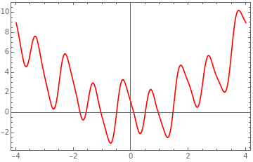
Plotting f(t) shows that this function has many local minima.
In[]:=
f[x_]:=0.5x^2+Cos[Pix]-2Sin[2Pix]+Cos[3Pix]Sin[Pix]
In[]:=
plt1=Plot[f[x],{x,-4,4},PlotStyleRGBColor[1,0,0],FrameTrue]
Out[]=
Using built-in functions of Mathematica, one finds several solutions and is not sure if he has found the global minimum which is obtained for x = -0.711232 and f(x) = -3.0233.
In[]:=
Minimize[f[x],x]
Out[]=
{-2.46045,{x1.27387}}
In[]:=
NMinimize[f[x],{x,-4,4}]
Out[]=
{-3.0233,{x-0.711232}}
In[]:=
NMinimize[f[x],{x,-2,2}]
Out[]=
{-3.0233,{x-0.711232}}
In[]:=
FindMinimum[f[x],{x,-2,2}]
Out[]=
{-0.70954,{x-1.66884}}
Simulated annealing gives the global minimum xbest and fbest=f(xbest).
In[]:=
X=0
Out[]=
0
In[]:=
fbest=f[X]
Out[]=
1.
In[]:=
M=0.5;
In[]:=
kT0=100;
In[]:=
For[k=1,k<11,{x=(Random[]-0.5)*8,F=f[x],For[j=1,j<10^4,{kT=kT0*(10^4+1-j)/10^4,newx=x+(Random[]-0.5)*M,newf=f[newx],p=Min[{1,Exp[-(newf-F)/kT]}],u=Random[],If[p≥u,{x=newx,F=newf}],j++}],sol=FindMinimum[f[t],{t,x}],F=sol[[1]],x=t/.sol[[2]],If[F<fbest,{xbest=x,fbest=F}],k++}]
In[]:=
fbest
Out[]=
-3.0233
In[]:=
xbest
Out[]=
-0.711232
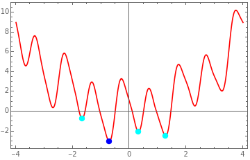
Mathematica built-in functions have found several local minima.
The global minimum found using simulated annealing is the dark blue dot.
The global minimum found using simulated annealing is the dark blue dot.
In[]:=
Show[plt1,Graphics[{RGBColor[0,0,1],PointSize[0.025],Point[{xbest,fbest}],RGBColor[0,1,1],PointSize[0.025],Point[{0.31758853903658163,-2.0607196324911374}],Point[{1.2738706370162356,-2.4604469522330414}],Point[{-1.6688381950990252,-0.7095400263875662}]}]]
Out[]=