Compiling different models of computation into hypergraph rewriting systems
by Utkarsh Bajaj
University of Waterloo
by Utkarsh Bajaj
University of Waterloo
By computational irreducibility, it is well known that Hypergraph rewriting systems are Turing complete i.e. they can compute any Turing-computable function. The goal of this project is to interpret a model of computation (such as a Turing Machine with imperative algorithms or functional lambda calculus) as a hypergraph rewriting system. For example, just as we can interpret a DFA (deterministic finite automaton) using a Turing machine with a set of states, a tape alphabet, and transition functions, we can interpret a DFA using a Hypergraph rewriting system with an initial Hypergraph and replacement rule. The first goal of this project is make a function that takes in a finite state machine and outputs the “equivalent” Hypergraph rewrite rule with an initial hypergraph (the input). The second goal of this project is to extend the same to imperative machines like Turing machines and register machines.The third goal of this project is to get the intuition for how we might formally define the notion of computability on Hypergraph rewriting systems, by creating a compiler from a high level Turing-complete functional language (called “Faux Racket”), which is defined below.
Section 0: Definitions, speculations, and some preliminary results
Section 0: Definitions, speculations, and some preliminary results
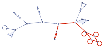
To get started, let’s formally define hypergraph rewriting systems as a computational system, as is used in the Wolfram physics project literature [1].
◼
Definition (Wolfram Model Hypergraph). A wolfram model hypergraph/hypergraph, denoted , is a finite collection of hyperedges (ordered): .
H=(V,E)
E⊂(V)\∅
◼
Definition (Update rule). An update rule, denoted , for a spatial hypergraph is an abstract rewriting rule of the form -> in which a subhypergraph matching pattern is replaced by a distinct subhypergraph matching pattern .
R
H=(V,E)
H
1
H
2
H
1
H
2
◼
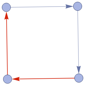
Note that the word distinct is important here. That’s the reason why the multiway evolution graph is acyclic for a wolfram model system.
◼
Definition (HRS). A hypergraph rewriting system is a set where is a set of hypergraphs is non-symmetric binary relation defined using the update rule.
HRS
(H,->)
H
->
◼
Note: the set will not be finite in most cases.
H
◼
Definition (Multiway Evolution Graph). A multiway evolution graph of an HRS, denoted is a directed acyclic graph (represents the evolution a generally non-confluent abstract rewriting system ) in which each vertex corresponds to a hypergraph and in which the directed edge exists iff there is a rewrite rule application transforming into , where .
G
multiway
(A,->)
a->b
a
b
a,b∈A
◼
Definition (Path). There is a path from a vertex to vertex if . There is a maximal path between and if and . We denote this by .
s
e
se
*
->
s
e
se
*
->
(∀h∈H)¬(e->h)
se
◼
It is obvious if there is a maximal path in the multiway system for a particular vertex, then there is a maximal path in that multiway system with as the starting vertex (we can merely trace back).
G
◼
There is a subtlety here which is obvious mathematically but not obvious for our intuition: a HRS is where is a set of hypergraphs. We define the binary relation between hypergraphs by seeing that if a single application of an update rule can transform one hypergraph into another hypergraph. However, we are only considering hypergraphs in the set . So if there is a rule that transforms one hypergraph into another hypergraph which is not in the set , they cannot be related because the binary relation is only defined on the set . So we should think of this as just a set with a binary relation on it, not really update rules: update rules generate the binary relation.
(H,->)
H
H
H
H
◼
Definition (Halting set). Let be an HRS. Then is in the halting set of an HRS , denoted , iff there exists a maximal path in the multiway evolution graph for ⧦ for some . If is not in the halting set, then it means that every path in the multiway system is non-maximal i.e. it doesn’t stop. We say that in this case.
(H,->)
G∈H
(H,->)
Ω(H)
G
GG'
G'∈G
G∈H
G↑
◼
Note that maximal paths are defined in the multiway system. If a hypergraph is not in an halting set, then it means that every path through the multiway system doesn’t stop running. So yes, there is no maximal path in the multiway system. Because if there is, then the initial hypergraph will be in the halting set.
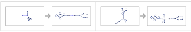
To understand how hypergraph rewriting works in the Wolfram language, refer to [2]. Now, we might come up with a intuitive definition for what it means for a HRS to simulate a Turing machine. First, let’s define what it means by saying “the tape at some time ):
t
◼
Definition (Tape at time ). Let be a Turing machine where is a finite set of internal states, is the finite tape alphabet, is the halting state, and is the initial state. Let be the initial tape (where to the left and right we have 0s). The tape at time , denoted , is defined inductively. . Then where where for any word is the new word produced on the tape after one application of the transition function.
t∈
T=(Q,Γ,δ,,)
q
halt
q
0
Q
Γ
q
halt
q
0
w∈
*
Γ
t
T(t)
T(1)=w
T(t+1)=δ(T(t))
t>=1
δ(w)
w
Now, the definition of a HRS simulating a Turing Machine.
◼
Definition (Hypergraph rewriting system simulates a Turing machine). Let be a Turing machine where is a finite set of internal states, is the finite tape alphabet, is the halting state, and is the initial state. Let be a hypergraph rewriting system. Then simulates if , such that
T=(Q,Γ,δ,,)
q
halt
q
0
Q
Γ
q
halt
q
0
(H,->)
(H,->)
T
∃f
f:->H
*
Γ
1
.∀w∈Ω(T)
f(w)G'
G'∼f(w')
w'=T(w)↓
2
.∀w∈\Ω(T)
*
Γ
(∀N∈)(∃n>=N)f(w)
->
n
G
n
G
n
It should be the case that if the HRS can simulate any Turing machine , then it should be able to compute any partial recursive function under a suitable definition of computability. Defining a precise notion of computability for hypergraphs that is able to leverage its flexibility and is most “suited” for hypergraphs is one of the future goals of the project. However, a tentative definition has been produced below (we represent as cyclic graph).
(H,->)
T
n∈
th
(n+1)
◼
Definition (One parameter family of maps )
χ
t
We first define a few graphs like these.
In[]:=
cyclicgraph[n_]:=If[n0,{{0,0}},Join[Table[{i,i+1},{i,0,n-1}],{{n,0}}]]
In[]:=
cyclicgraph[n_,start_]:=If[n0,{{start,start}},Join[Table[{i+start,i+1+start},{i,0,n-1}],{{n+start,start}}]]
In[]:=
convertToStringRule[rule_]:=rule/.(Table[i"x"<>ToString[i],{i,Min[#1],Max[#1]}]&)[Join[rule〚1〛,rule〚2〛]]
In[]:=
χ1[n_]:=cyclicgraph[n,5](*CYCLICGRAPHS*)
In[]:=
χ2[n_]:=Join[cyclicgraph[n,4],stateGraph[0],{{3,4}}](*CYCLICGRAPHSWITH"STATE"ATTACHED*)
In[]:=
χ3[n_,k_]:=Ifk==1,cyclicgraph[n],Joincyclicgraph[n],Floor,n+1,n+1+#&[χ3[n,k-1]](*CYCLICGRAPHSSTRINGEDTOGETHER*)
n
2
χ4[n_,k_]:=Ifk==1,χ2[n],JoinJoincyclicgraph[n],Floor,n+1,n+1+#&[χ3[n,k-1]]+4,stateGraph[0],{{3,4}}(*CYCLICGRAPSHSTRINGEDTOGETHERWITHSTATEATTACHEDTOFIRSTONE(INONEEND)*)
n
2
In[]:=
χ[2,{a_,b_},state_]:=Join[cyclicgraph[a],{{Floor[a/2],a+1}},cyclicgraph[b,a+1],JoinState[a+b+1,Floor[a/2],state]]
In[]:=
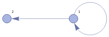
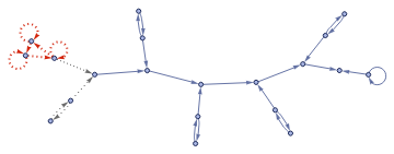
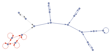
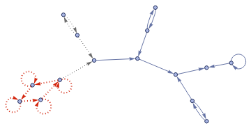
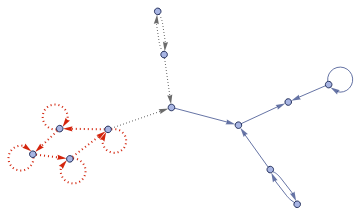
ResourceFunction["WolframModelPlot"][χ2[10],VertexLabels->Automatic]
Out[]=
In[]:=
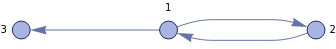
ResourceFunction["WolframModelPlot"][χ3[10,3],VertexLabels->Automatic]
Out[]=
In[]:=
χ[2,{a_,b_},state_]:=Join[cyclicgraph[a],{{Floor[a/2],a+1}},cyclicgraph[b,a+1],JoinState[a+b+1,Floor[a/2],state]]
χ2[2,{2,3},2]
In[]:=
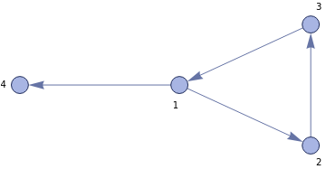
ResourceFunction["WolframModelPlot"][χ[2,{2,3},2],VertexLabels->Automatic]
Out[]=
◼
Definition (Partial computable). A partial function is said to partial computable if there exists an HRS (where is a set of hypergraphs and is a binary relation on ) and one map out of the one-parameter family of maps defined above such that for which is defined, and , where is isomorphic to cyclic graph. Also, for every outside the domain of , .
f:->
k
(H,->)
H
->
H
χ:->H
k
∀n∈
f(n)
χ(n)∈Ω(H)
χ(n)G
G
th
f(n)
n
f
χ(n)
Now that we have a notion of computability, we can prove a few theorems/lemmas.
◼
Lemma. The successor function is partial computable
n↦n+1
◼
Proof. Let be . Then, we can show that for all , (n) under the rule successor:
χ
χ
2
n
χ
2
C
n+1
In[]:=
successor={{x1,x2},{x2,x3},{x3,x},{x3,x3},{x2,x2},{x1,x1},{x1,x4},{x4,x5}}<->{{x4,x6},{x6,x5}};
In[]:=
FindWolframModelProof[χ2[2]<->cyclicgraph[3],successor]
Out[]=
ProofObject
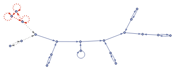
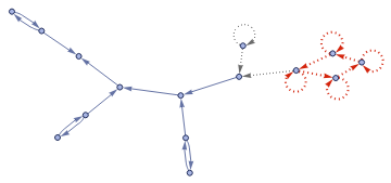
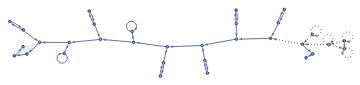
where the FindWolframModelProof function is defined in the Appendix, taken directly from [3]. We can visualise the evolution:
In[]:=
ResourceFunction["WolframModel"][{{x1,x2},{x2,x3},{x3,x},{x3,x3},{x2,x2},{x1,x1},{x1,x4},{x4,x5}}->{{x4,x6},{x6,x5}},χ2[2],"EventsStatesPlotsList"]
Out[]=
,
◼
Lemma. The identity function is computable
n↦n
◼
Proof. Let be . The rule is the empty rule.
χ
χ
1
In[]:=
identity={};
◼
Lemma. The function is computable.
n↦0
◼
Proof. Let by . The rule is constant 0, given below:
χ
χ
1
In[]:=
constant0=convertToStringRule[{{1,2},{2,3}}<->{{1,3}}];
In[]:=
FindWolframModelProof[χ1[10]<->cyclicgraph[0],constant0]
Out[]=
ProofObject
◼
Lemma. The function where is computable.
n↦kn
k∈
◼
Proof. Let χ by (with the second argument being . Note that we can enumerate all of these). The rule is:
χ
3
k
In[]:=
multiplybyconstant=convertToStringRule/@{{{1,2},{3,2},{3,4}}<->{{1,4},{3,2},{5,6},{6,7},{7,5},{5,5},{6,6},{7,7},{5,1}},{{1,2},{2,3},{3,1},{1,1},{2,2},{3,3},{3,4},{4,5},{5,6}}<->{{4,6}}};
In[]:=
FindWolframModelProof[χ3[10,3]<->cyclicgraph[30],multiplybyconstant]
Out[]=
ProofObject
◼
Lemma. The function is computable.
(,)↦+
n
1
n
2
n
1
n
2
◼
Proof. let’s choose as the initial graph. The rule is as follows:
χ[2,{,},0]
n
1
n
2
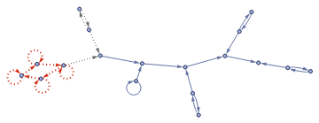
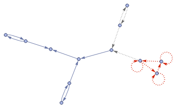
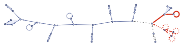
In[]:=
add2[state_]:=convertToStringRule/@{Join[{{2,1},{2,3},{4,3}},JoinState[4,2,state]]->Join[{{4,1},{2,3}},JoinState[4,2,state+1]],Join[{{1,2},{2,3}},JoinState[3,1,state+1]]->{{1,3}}}
In[]:=
ResourceFunction["WolframModel"][add2[0],χ[2,{4,5},0],3,"EventsStatesPlotsList"]
Out[]=
,
,
These results provide some intuition on how we might define computability on hypergraph rewriting systems. However, I think that there are better ways of defining computability. Proving that computability on hypergraph rewriting systems is closed under function composition, primitive recursion, and minimalization is non-trivial. That’s why I decided to compile different existing models of computation into hypergraph rewriting systems and see which ones are the most “natural” to hypergraph rewriting systems because it is difficult, a priori, to come up with a definition of computability of partial functions that leverage the flexibility of hypergraph rewriting systems. So, I’ve decided to explicitly convert Finite state machines, single-tape Turing machines, register machines, and “Faux racket” into hypergraph rewriting systems. The conclusion is that that hypergraph rewriting systems, although Turing-complete like other models, are “powerful”/efficient enough to compile a functional language like Faux racket with only very minimal set of replacement rules. On a surface level, it has been realised that hypergraph rewriting systems are more efficient than a single-tape Turing machines for the same reason that multi-tape Turing machines are more efficient that single tape Turing machines. More precisely, the notion of concurrent programming is very natural to an HRS. For example, as opposed to how an ordinary compiler might create stack frames to perform computations sequentially, in hypergraph rewriting systems, we can a “new stack” itself by creating a disconnected hypergraph, and performing computations there. In this way, we can increase the “dimension” of an HRS to support concurrent programming whenever possible. These ideas are elaborated upon in the last section on faux racket to hypergraph conversion. It will be apparent to the reader that when we will simulate Turing machines and Register machines using hypergraph rewriting, we only use a very specific class of hypergraphs and rewrite rules.
Section 1: Converting FSMs into Hypergraph rewriting
Section 1: Converting FSMs into Hypergraph rewriting
Subsection 1. DFAs
Subsection 1. DFAs
Given a DFA , we need to convert it into the associated hypergraph rewriting system i.e. an initial hypergraph and a collection of rules.
(Q,Σ,δ,,F)
q
0
It is quite trivial to convert DFAs to hypergraph rewriting. A DFA consists of a number of states and an alphabet. So we begin by defining simple graphs for symbols in an alphabet :
Σ
In[]:=
alphabetGraphHelper[n_]:=If[n==0,{{1,1},{1,2}},If[n==1,{{1,2},{2,1}},Module[{x},x=Last[#][[1]]&[alphabetGraphHelper[n-1]];Join[Drop[#,-1],{{x,x+1},{x+1,1}}]&[alphabetGraphHelper[n-1]]]]]
In[]:=
alphabetGraph[n_]:=If[n==0,{{1,1},{1,2}},Append[alphabetGraphHelper[n],{1,n+2}]]
In[]:=
ResourceFunction["WolframModelPlot"][#,VertexLabels->Automatic]&/@Table[alphabetGraph[n],{n,0,8}]
Out[]=
,
,
,
,
,
,
,
,
In[]:=
stateGraph[n_]:=Join[Table[{i,i},{i,1,n+3}],Table[{i,i+1},{i,1,n+3-1}],{{n+3,1}}]
In[]:=
graphToHypergraph[g_]:=g/.x_Integery_Integer{x,y}
In[]:=
concatenategraphs[g1_,g2_]:=graphToHypergraph[Join[{Max[VertexList[g1]]Max[VertexList[#]]},#]]&[EdgeList[GraphDisjointUnion[g1,g2]]]
In[]:=
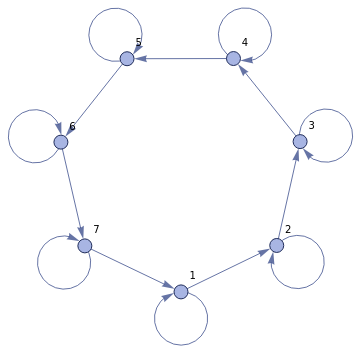
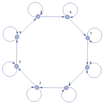
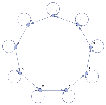
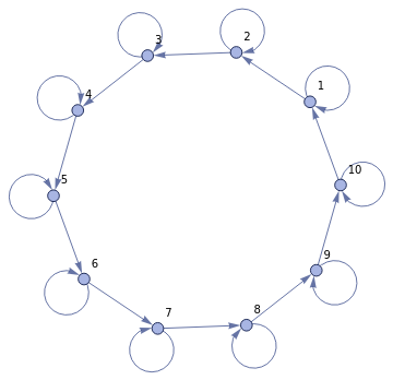
ResourceFunction["WolframModelPlot"][#,VertexLabels->Automatic]&/@Table[stateGraph[n],{n,1,8}]
Out[]=
,
,
,
,
,
,
,
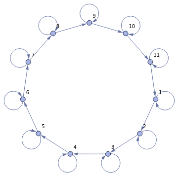
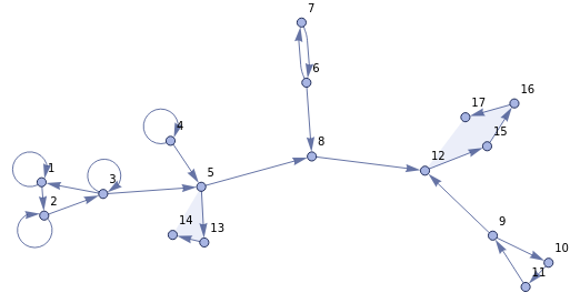
The reason why we have loops on state graphs is to ensure that when we apply rewrite rules, we have no overlapping subhypergraphs with state graphs. Essentially, we have to obey 4 conditions: no 2 distinct state graphs are subgraphs of each other, no 2 distinct alphabet graphs are subgraphs of each other, a state graph is not a subgraph of any alphabet graph, and any alphabet graph is not a subgraph of any state graph. The above encoding satisfies these conditions. The reason why we have starting iterating the state graphs from 3 is preuly due to some edge cases that need to be handled.
At a particular step, there will be all types of rewrite rules. But we only want to make sure only one rewrite rule will be applied that brings the DFA onto the first step. That’s where we can use graph concatenation. For instance, let’s say is represented by hypergraph and 0 is represented by hypergraph . Then, we will also have hypergraphs for the states and represented by and . Then, if the input to the DFA is 1011, then the input hypergraph would where χ and ⊕ are binary operators on the space of hypergraphs. Then, the first transition function applied would be . There should be a rewrite rule corresponding to this transition function that brings the hypergraph into . And so on. The rule corresponding to the transition function should apply iff the first graph is of the form where can be anything. Then, we have a finite rewrite rule as well that applies to any state graph but not any other graph. Thus, we have to satisfy the following conditions:
1
A
1
A
0
q
0
q
1
S
0
S
1
(χ)⊕⊕⊕
S
0
A
1
A
0
A
1
A
1
δ(,1)
q
0
R
01
(χ)⊕⊕⊕
S
0
A
1
A
0
A
1
A
1
(χ)⊕⊕
S
1
A
0
A
1
A
1
δ(,_)
q
i
χ
S
i
A
j
j
◼
Any state graph should not be equal to or be a subgraph of other state graph where .
S
i
S
j
i≠j
◼
Any state graph should not be equal or be a subgraph of any other where . Also, should not be a subgraph of any other state graph .
S
i
A
j
j≠i
A
j
S
i
◼
Note that this implies that no graph χ is a subgraph or is equal to the graph χ where .
S
i
A
j
S
k
A
l
(i,j)≠(k,l)
◼
The rule , corresponding to the transition function i.e. when in state and alphabet should apply iff the hypergraph is of the form
R
ij
δ(i,j)
q
i
j
χ⊕⊕⊕⊕..
S
i
A
j
A
i
1
A
i
2
A
i
3
In[]:=
concatenategraphs[g1_,g2_]:=graphToHypergraph[Join[{Max[VertexList[g1]]Max[VertexList[#]]},#]]&[EdgeList[GraphDisjointUnion[g1,g2]]]
In[]:=
initialWordToHypergraphHelper[word_List,acc_]:=If[word=={},acc,initialWordToHypergraphHelper[Drop[word,1],concatenategraphs[acc,alphabetGraph[word[[1]]]]]]
In[]:=
initialWordToHypergraph[word_List]:=initialWordToHypergraphHelper[Drop[word,1],concatenategraphs[stateGraph[0],alphabetGraph[word[[1]]]]]
In[]:=
Graph[initialWordToHypergraph[{0,1,2,3,4,5,5,2,2,3}],VertexLabels->Automatic]
Out[]=
So we can convert any word into an initial hypergraph.
In[]:=
DFARule[{stateI_,alphabet_,stateF_}]:=((#->ReplaceAll[stateGraph[stateF],Join[Table[i->Max[VertexList[#]]+i,{i,1,stateF+3-1}],{stateF+3->Max[VertexList[#]]}]])&)[concatenategraphs[stateGraph[stateI],alphabetGraph[alphabet]]]
The following represents :
δ(,2)=
q
1
q
0
In[]:=
RulePlot[ResourceFunction["WolframModel"][DFARule[{1,2,0}]],VertexLabels->Automatic]
Out[]=
The preserved vertex is the link between the symbol (in ) to the left and the symbol to the right (in ).
Σ
Σ
In[]:=
DFAtoHypergraph[rules_List,word_]:=ResourceFunction["WolframModel"][Table[DFARule[i],{i,Map[Join[#[[1]],#[[2]]]&,(rules/.Rule->List)]}],initialWordToHypergraph[word],Length[word],"EventsStatesPlotsList"]
In[]:=
DFAtoHypergraph[{{0,0}->{0},{0,1}->{1},{1,0}->{0},{1,1}->{1}},{0,1,1,1,1,1,0}]
Out[]=
,
,
,
,
,
,
,
The DFA is constructed in such a way so that if the final symbol is 0, then the final state is 0. And if the final symbol is 1, the final state is 1. We can see that the above holds.
In[]:=
DFAtoHypergraph[{{0,0}->{0},{0,1}->{1},{1,0}->{0},{1,1}->{1}},{0,1,1,0,1,1,1}]
Out[]=
,
,
,
,
,
,
,
So, DFAs are converted to Turing machines in a pretty direct manner. The state of a Turing machine is represented by a subgraph that attaches itself to the symbol it is currently reading, and then moves to the right to the next symbol. It continues to do so until there are no symbols left to read, and we end up with the final state.
One may ask: why do we need a state subgraph? All models of finite state machines, Turing machines, and register machines are sequential in nature. So states in these models are used to impose a definite order of evaluation. In hypergraph rewriting systems, the analogy to a state is this subgraphs that moves along the hypergraph to dictate the application of a rule, to effectively impose a definite updating order. From here, it is also pretty easy to implement Turing machines because it is similar to a DFA, except that the state subgraphs can move either to the left or right, and can change the symbols.
Subsection 2. NFAs
Subsection 2. NFAs
Section 2. Converting Turing-complete Imperative machines into Hypergraph rewriting
Section 2. Converting Turing-complete Imperative machines into Hypergraph rewriting
Subsection 1. Turing Machines
Subsection 1. Turing Machines
We use the same approach as in DFAs.
In[]:=
initialTapeToHypergraph[word_List]:=Module[{x,y,z},x=initialWordToHypergraph[word];y=Max[VertexList[concatenategraphs[stateGraph[0],alphabetGraph[word[[1]]]]]];z=Max[VertexList[x]];Join[x,{{y,z+1,z+2},{z,z+3,z+4,z+5}}]]
In[]:=
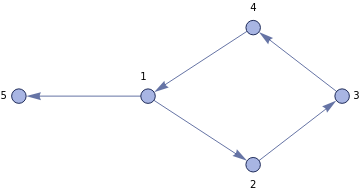
ResourceFunction["WolframModelPlot"][initialTapeToHypergraph[{0,1,2}],VertexLabels->Automatic]
Out[]=
The hyperedges at the ends indicate the left and right ends of the tape. I have introduced those so that if the head wants to move to the right, beyond the currently defined tape, there will be a special rewrite rule that will create the 0 symbol and join it to the existing tape, extending the right hyperdge to indicate the new end of the tape. Same goes for the left hyperedge.
In[]:=
TuringRule[{stateI_,symbolI_}->{stateF_,symbolF_}]:={#->Join[JoinState[Max[VertexList[#]],Max[VertexList[#]],stateF],JoinAlphabet[stateF+3+Max[VertexList[#]],Max[VertexList[#]],symbolF]]}&[concatenategraphs[stateGraph[stateI],alphabetGraph[symbolI]]]
In[]:=
TuringRule[{stateI_,symbolI_}->{stateF_,symbolF_,offset_}]:=If[offset==0,TuringRule[{stateI,symbolI}->{stateF,symbolF}],Module[{x=Max[VertexList[#]]},If[offset==1,(*theedgecases---literally*){Join[#,{{x,x+1}}]->Join[JoinState[x+1,x+1,stateF],JoinAlphabet[stateF+3+x+1,x,symbolF],{{x,x+1}}],Join[#,{{x,x+1,x+2,x+3}}]->Join[JoinState[x+4,x+4,stateF],JoinAlphabet[stateF+3+x+4,x,symbolF],JoinAlphabet[stateF+3+x+4+symbolF+2,x+4,0],{{x,x+4},{x+4,x+4+stateF+3+symbolF+6,x+4+stateF+3+symbolF+7,x+4+stateF+3+symbolF+8}}]},If[offset==-1,{Join[#,{{x+1,x}}]->Join[JoinState[x+1,x+1,stateF],JoinAlphabet[stateF+3+x+1,Max[VertexList[#]],symbolF],{{x+1,x}}],Join[#,{{x,x+1,x+2}}]->Join[JoinState[x+5,x+3,stateF],(*jointhestateatx+3*)JoinAlphabet[stateF+3+x+5,x,symbolF],(**)JoinAlphabet[stateF+3+x+5+symbolF+2,x+3,0],{{x+3,x},{x+3,x+4,x+5}}]}]]]&[concatenategraphs[stateGraph[stateI],alphabetGraph[symbolI]]]]
In[]:=
RulePlot[ResourceFunction["WolframModel"][TuringRule[{0,1}->{1,4,-1}]]]
Out[]=
In[]:=
HaltRule[state_]:=(Join[#,{{1,Max[VertexList[#]]+1}}]->{})&[stateGraph[state]]
In[]:=
TuringToHypergraph[rules_,qHalt_,word_,steps_]:=ResourceFunction["WolframModel"][Join[Flatten[TuringRule/@rules,1],{HaltRule[qHalt]}],initialTapeToHypergraph[word],steps,"EventsStatesPlotsList"]
Here are a few examples:
In[]:=
TuringToHypergraph[{{0,0}->{0,0,1},{0,1}->{0,0,1}},1,{0,1,1,1,1,0,1,0,1},5]
Out[]=
,
,
,
,
,
Another example:
In[]:=
TuringToHypergraph[{{0,1}->{3,0},{0,0}->{1,1,-1},{1,1}->{1,1,1},{1,0}->{1,0,1}},2,{0,1,1,2},10]
Out[]=
,
,
,
,
,
The reader is encouraged to play around with this code and get an intuition for how we have compiled from hypergraph rewriting systems to Turing machines. The rewrite rules are self explanatory and can be understood by using Rule Plot, as shown in the previous example. Note that we have used the same encoding for Turing machines.
Register machines
Register machines
◼
Definition (Referring to a State). A register refers to state if state is of the form or .
R
i
S
j
S
j
(i,+,j)
(i,-,k,l)
In[]:=
numberGraph[start_,n_]:=If[n0,{{start,start}},Join[Table[{start+i-1,start+i},{i,1,n}],{{start+n,start}}]]
In[]:=
JoinState[n_,m_,stateF_]:=Join[ReplaceAll[stateGraph[stateF],Table[i->n+i,{i,1,stateF+3}]],{{stateF+3+n,m}}]
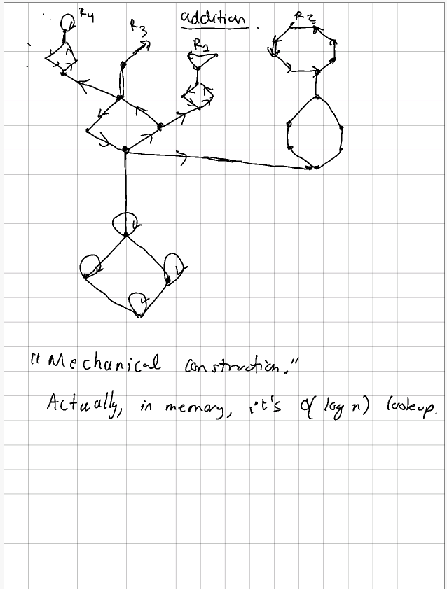
I am using an hypergraph subgraph that “connects” to other registers. This is because one register can be referred to by Multiple instructions. So when we have a particular instruction, we can go to different registers depending on the type of state. To avoid interference, each instruction will correspond to a particular exit route (non-isomorphic).
For example:
In[]:=
nHypergon[n_,m_]:={Join[Range[m,m+n-1],{m}]}
This takes in a state number , integers where (), and the instruction . represents the size of the attached to this register i.e. the number of states referred to by this register. The number tells us what state is currently attached to this register (each state referred to by this register has a unique such --this is the entire point).
"state"
n,p
1<=p<=n
n>=1
{i_,"+",j_}
n
n-hypergron
p
p
In[]:=
RegisterRule2[state_,n_,p_,{i_,"+",j_}]:=Module{x,m},x=stateGraph[state];m=Max[VertexList[x]];Ifn<=4,(*since1<=p<=n,(n>=1),m+p*)If[j==0,{Join[x,{{m,m+1},{m+1,m+2,m+3,m+4,m+1},{m+5,m+3},{m+5,m+6}}]->Join[JoinState[m+7,m+1,0],{{m+1,m+2,m+3,m+4,m+1},{m+p,m+7},{m+5,m+3},{m+5,m+8},{m+8,m+6}}]},{Join[x,{{m,m+1},{m+1,m+2,m+3,m+4,m+1},{m+5,m+3},{m+5,m+6},{m+p,m+7}}]->Join[JoinState[m+8,m+7,j],{{m+1,m+2,m+3,m+4,m+1},{m+p,m+7},{m+5,m+3},{m+5,m+8},{m+8,m+6}}]}],(*n>=5*)Ifj==0,Joinx,{{m,m+1}},nHypergon[n,m+1],m+n+1,m+Floor+1,{m+n+1,m+n+2}->JoinnHypergon[n,m+1],m+n+1,m+Floor+1,{m+n+1,m+n+4},{m+n+4,m+n+2},JoinState[m+n+5,m+1,j],Joinx,{{m,m+1}},nHypergon[n,m+1],m+n+1,m+Floor+1,{m+n+1,m+n+2},{m+p,m+n+3}->JoinnHypergon[n,m+1],m+n+1,m+Floor+1,{m+n+1,m+n+4},{m+n+4,m+n+2},{m+p,m+n+3},JoinState[m+n+4,m+n+3,j]
n
2
n
2
n
2
n
2
In[]:=
In[]:=
RegisterToAssocHelper[stateReg_,instructions_,acc_,num_]:=Module[{instr,list},instr=instructions[[1]];(*Print[acc];*)list=Lookup[acc,instr[[1]]];If[instructions=={},acc,If[instr[[2]]=="+",If[instr[[3]]==0,RegisterToAssocHelper[stateReg,Drop[instructions,1],Append[acc,instr[[1]]->Join[list,{{num,{0,0}}}]],num+1],RegisterToAssocHelper[stateReg,Drop[instructions,1],Append[acc,instr[[1]]->Join[list,{{num,{instr[[3]],Lookup[stateReg,instr[[3]]]}}}]],num+1]],If[instr[[3]]==0&&instr[[4]]==0,RegisterToAssocHelper[stateReg,Drop[instructions,1],Append[acc,instr[[1]]->Join[list,{{num,{0,0},{0,0}}}]],num+1],If[instr[[3]]==0,RegisterToAssocHelper[stateReg,Drop[instructions,1],Append[acc,instr[[1]]->Join[list,{{num,{instr[[4]],Lookup[stateReg,instr[[4]]]},{0,0}}}]],num+1],If[instr[[4]]==0,RegisterToAssocHelper[stateReg,Drop[instructions,1],Append[acc,instr[[1]]->Join[list,{{num,{0,0},{instr[[3]],Lookup[stateReg,instr[[3]]]}}}]],num+1],RegisterToAssocHelper[stateReg,Drop[instructions,1],Append[acc,instr[[1]]->Join[list,{{num,{instr[[4]],Lookup[stateReg,instr[[4]]]},{instr[[3]],Lookup[stateReg,instr[[3]]]}}}]],num+1]]]]]]]
In[]:=
countZeros[list_]:=If[list=={},0,If[list[[1]]==0,countZeros[Drop[list,1]]+1,countZeros[Drop[list,1]]]]
In[]:=
lengthRegister[registerAssoc_]:=If[registerAssoc=={},0,If[Length[registerAssoc[[1]]]==3,lengthRegister[Drop[registerAssoc,1]]+2-countZeros[{registerAssoc[[1]][[2]][[1]],registerAssoc[[1]][[3]][[1]]}],lengthRegister[Drop[registerAssoc,1]]+1-countZeros[{registerAssoc[[1]][[2]][[1]]}]]]
In[]:=
RegisterToAssoc[instructions_]:=RegisterToAssocHelper[AssociationMap[(instructions[[#]][[1]])&,Range[Length[instructions]]],instructions,AssociationMap[{}&,DeleteDuplicates[#[[1]]&/@instructions]],1]
In[]:=
registerGraph[value_,nref_,start_]:=If[nref<=4,Join[{{start,start+1,start+2,start+3,start},{start+4,start+2}},numberGraph[start+4,value]],Join[{Range[start,start+nref-1]},{{start+nref-1,start},{start+nref,start+Floor[nref/2]}},numberGraph[start+nref,value]]]
In[]:=
registerGraphs[initRegValues_,keys_,values_,acc_]:=If[keys=={},<||>,Join[<|keys[[1]]->#|>,registerGraphs[initRegValues,Drop[keys,1],Drop[values,1],Max[#]+1]]&[registerGraph[Lookup[initRegValues,keys[[1]]],lengthRegister[values[[1]]],acc]]]
In[]:=
initialRMtoHypergraph[initRegValues_,instructions_,assoc_,RegisterGraphAssoc_]:=Module[{j,connectRegisters},connectRegisters[register_,acc_,num_]:=If[register=={},{},If[Length[register[[1]]]==2,If[register[[1]][[2]][[1]]==0,connectRegisters[Drop[register,1],acc,num],Join[{{num+acc-1,Min[Lookup[RegisterGraphAssoc,register[[1]][[2]][[2]]]]}},connectRegisters[Drop[register,1],acc+1,num]]],(*iflength=3*)If[register[[1]][[2]][[1]]==0&®ister[[1]][[3]][[1]]==0,connectRegisters[Drop[register,1],acc,num],If[register[[1]][[2]][[1]]==0,Join[{{num+acc-1,Min[Lookup[RegisterGraphAssoc,register[[1]][[3]][[2]]]]}},connectRegisters[Drop[register,1],acc+1,num]],If[register[[1]][[3]][[1]]==0,Join[{{num+acc-1,Min[Lookup[RegisterGraphAssoc,register[[1]][[2]][[2]]]]}},connectRegisters[Drop[register,1],acc+1,num]],Join[{{num+acc-1,Min[Lookup[RegisterGraphAssoc,register[[1]][[2]][[2]]]]},{num+acc,Min[Lookup[RegisterGraphAssoc,register[[1]][[3]][[2]]]]}},connectRegisters[Drop[register,1],acc+2,num]]]]]]];Join[Flatten[Table[connectRegisters[Lookup[assoc,i],1,Min[Lookup[RegisterGraphAssoc,i]]],{i,Keys[assoc]}],1],Flatten[Values[RegisterGraphAssoc],1]]]
In[]:=
ruleRegister[n_,register_,acc_]:=If[register=={},{},If[Length[register[[1]]]==2,If[register[[1]][[2]][[1]]==0,Join[RegisterRule2[register[[1]][[1]],n,acc,{i,"+",register[[1]][[2]][[1]]}],ruleRegister[n,Drop[register,1],acc]],Join[RegisterRule2[register[[1]][[1]],n,acc,{i,"+",register[[1]][[2]][[1]]}],ruleRegister[n,Drop[register,1],acc+1]]],(*length=3.example:register[[1]]={4,{0,0},{5,1}}*)If[register[[1]][[2]][[1]]==0&®ister[[1]][[3]][[1]]==0,Join[RegisterRule2[register[[1]][[1]],n,acc,{i,"-",0,0}],ruleRegister[n,Drop[register,1],acc]],If[register[[1]][[2]][[1]]==0,Join[RegisterRule2[register[[1]][[1]],n,acc,{i,"-",register[[1]][[3]][[1]],0}],ruleRegister[n,Drop[register,1],acc+1]],If[register[[1]][[3]][[1]]==0,Join[RegisterRule2[register[[1]][[1]],n,acc,{i,"-",0,register[[1]][[2]][[1]]}],ruleRegister[n,Drop[register,1],acc+1]],Join[RegisterRule2[register[[1]][[1]],n,acc,{i,"-",register[[1]][[3]][[1]],register[[1]][[2]][[1]]}],ruleRegister[n,Drop[register,1],acc+2]]]]]]];
In[]:=
RMtoHypergraph[initRegValues_,instructions_,steps_]:=Module[{assoc,RegisterGraphAssoc,initialHypergraph},assoc=RegisterToAssoc[instructions];RegisterGraphAssoc=registerGraphs[initRegValues,Keys[assoc],Values[assoc],1];initialHypergraph=Join[#,JoinState[Max[#],Min[Lookup[RegisterGraphAssoc,instructions[[1]][[1]]]],1]]&[initialRMtoHypergraph[initRegValues,instructions,assoc,RegisterGraphAssoc]];ResourceFunction["WolframModel"][Join[Flatten[Table[ruleRegister[lengthRegister[#],#,1]&[Lookup[assoc,i]],{i,Keys[assoc]}],1],{Join[stateGraph[0],{{3,4}}]->{}}],initialHypergraph,steps,"EventsStatesPlotsList"]]
This is the code.
Add the contents of to , leaving unchanged. Here we are adding 10 and 7. Note that ist’s the same number of steps as a register machine. So yeah, I’ve actually physically implemented a register machine.
R
1
R
2
R
1
In[]:=
RMtoHypergraph[<|1->5,3->0,2->3|>,{{1,"-",2,4},{3,"+",3},{2,"+",1},{3,"-",5,0},{1,"+",4}},70]

Out[]=
Section 3. Converting Faux Racket into Hypergraph Rewriting
Section 3. Converting Faux Racket into Hypergraph Rewriting
The language “Faux racket” is taken from the CS 146 class (Program design) at the University of Waterloo. It’s grammar is defined as the following:
expr = num | var | (+ expr expr) | (* expr expr) | (- expr expr) | (fun (var) expr) | (expr expr) | (ifzero expr expr expr) | (with ((var expr)) expr) | (rec ((var expr)) expr)
We will compile this into the following:
data ast = num | (Bin “+“ expr expr) | (Sub1 expr) | (Fun (var) expr) | (App ast ast var) | (IfZero ast ast ast) | (Rec ((var expr)) expr)
Appendix
Appendix
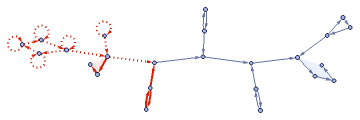
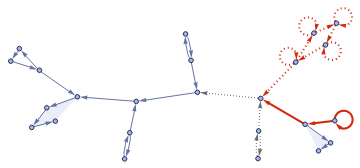
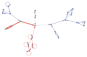
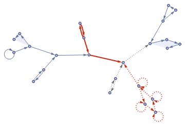
FindWolframModelProof [3]
FindWolframModelProof [3]
References
References
◼
[1]. Gorard, Jonathan. Some Relativistic and Gravitational Properties of the Wolfram Model.
◼
[2]. Wolfram, Stephen. A Class of Models with the Potential to Represent Fundamental Physics
◼
[3]. Gorard, Jonathan. FindWolframModelProof (Resource function)