Chromatin tends to form knots within the nucleus, which, without proper resolution by topoisomerases, can lead to cell death and mutation. However, the mechanism of this knot formation is poorly understood. Using a mechanical model, this project aims to simulate different knots along randomly moving DNA segments, and analyze the knots’ motion and size. We found that chromatin knots in this model are prone to rightward movement, size decreases, and are heavily influenced by the ratio of knot to chain length. These results provide further insight into DNA knot dynamics and can be applied to future drug development and nanotechnology.
Introduction
Introduction
Deoxyribonucleic acid (DNA) is a long polymer containing genetic information that is folded and replicated trillions of times each day. However, like any long polymer, it is inevitable that DNA tangles itself into a knot. In fact, DNA knots are fairly common in intracellular chromatin, where they are resolved by topoisomerase II and IV during replication. Even so, when these knots aren’t removed, they block DNA transcription and replication, induce apoptosis, and lead to a mutation rate three to four times higher than that of unknotted DNA. Therefore, studying the mechanism of DNA knot formation and movement is vital for understanding these causes of DNA damage.
In the nucleus, DNA exists as compact chromatin, where long chains of DNA are wrapped around histone proteins. Particularly, this chromatin has a tendency to randomly move, as dictated by the thermal fluctuations in its environment. During this random motion, chromatin links segments of DNA together by histone complexes, forming one long chain of several segments. This chain forms knots, which are not easily identifiable in vivo. Instead, in silico models are often used, where simulations can be run thousands of times.
The objective of this project was to take these conditions and simulate a knot along a randomly moving segment of chromatin. This chromatin is represented by a series of DNA segments (lines), and the knot within the chromatin will be studied to determine its overall displacement, size, and slack. While these were the main objectives, this project also aims to model the formation of a knot from a moving piece of chromatin, as well as model different kinds of knots. By analyzing the mechanical representation of this knot, we can gain insight into general knot dynamics and demonstrate an application of physics and knot theory to future drug development and DNA crystal structures.
Set-Up
Set-Up
The number of line segments in this series of DNA, and the number of frames in the animation:
In[]:=
n=30;timesteps=200;
In order to simulate DNA, we fixed two endpoints of DNA and maintained a constant length for each segment.
Fixed endpoints of DNA:
In[]:=
p1={-1,0,0};p2={1,0,0};ogPointDist=p2-p1;
A parameter for vertical displacement to allow slack:
In[]:=
vert=0.06;
Determining segment length:
In[]:=
dist=Norm[p2-p1];tempLength=dist/n;segLength=Sqrt[tempLength^2+vert^2];
Parameter for collision minimum distance based on segment length:
In[]:=
minDistance=Floor[segLength,0.01];
After which, basic variables for building the knot are constructed. To make a looser or more defined knot, the number of segments in the knot increases. Based on the knot’s number of segments, the length of straight DNA tails are determined.
Deciding knot and tail length:
In[]:=
knotSegmentCount=20;preEndIndex=Floor[(n-knotSegmentCount)/2-1];postStartIndex=Floor[(n+knotSegmentCount)/2+1];
Building the Chromatin Chain:
Building the Chromatin Chain:
For this project, our focus will be on the trefoil knot, one of the simplest and most common knots. Our model for chromatin involves a straight tail of DNA, the trefoil knot, and another straight tail of DNA. This ensures that the knot stays roughly in the middle, allowing it to move in either direction and avoid the ends.
Creating the First Chromatin Tail:
Creating the First Chromatin Tail:
In order to allow knot movement along the chromatin, the chromatin must be fairly loose, even when fixed to two endpoints. To maintain this looseness, a vertical displacement for slack is added to the initial tails, allowing the DNA to be longer than the distance between the fixed points. Using this, the tails of chromatin are built.
Creating the pre-knot DNA tail:
prePoints=Table[p1+(i/(n-1))*(ogPointDist)+{0,If[EvenQ[i],vert,-vert],0},{i,0,preEndIndex+1}];Graphics3D[Tube[prePoints],PlotRange->{{-1,-0.5},{-0.1,0.1},{-0.1,0.1}},Boxed->False]
Out[]=

Building a Left-Handed Trefoil Knot:
Building a Left-Handed Trefoil Knot:
Now, a knot may be created. As mentioned earlier, this project uses a trefoil knot. A trefoil knot is characteristic in that it has three crossings, and has chirality in a left-handed and right-handed version. A trefoil knot follows a parametric equation where x=sin(t)+2sin(2t), y=cos(t)-2cos(2t), z=-sin(3t). However, because this model simulates DNA, a linear strand of DNA, this parametric’s t is restricted from -π/8 to 49π/32 to allow a linear chain rather than a circular one.
Creating a list of knotSegmentCount points along the modified trefoil:
steps=Subdivide[-Pi/8,(49*Pi)/32,knotSegmentCount];rawPoints=Table[{Sin[t]+2*Sin[2*t],Cos[t]-2*Cos[2*t],-Sin[3*t]},{t,steps}];Graphics3D[Tube[rawPoints],PlotRange->All,Boxed->False]
Out[]=

While we now have regular line segments along the trefoil knot, they are not necessarily the same length as the segments on the pre-knot DNA. In order to maintain segment length, the vector directions of each knot segment is calculated, and scaled to the appropriate length. After which, the knot must be inserted into the rest of the DNA chain.
Calculating direction and scaling knot segments:
segments=Partition[rawPoints,2,1];unitVectors=Map[segLength*Normalize[#[[2]]-#[[1]]]&,Most[segments]];knotPoints=FoldList[Plus,rawPoints[[1]],unitVectors];Graphics3D[Tube[rawPoints],PlotRange->All,Boxed->False]
Out[]=

In order to insert the knot into the DNA chain, it must be moved such that the start and endpoints align with the ones based on the pre-knot DNA. This requires rotations and translation using vector math.
Calculating the desired start and end coordinates of the knot based on pre-knot DNA positions:
In[]:=
startAnchor=prePoints[[-1]];endAnchor=startAnchor+(knotSegmentCount/(n-1))*(p2-p1);
Calculating the vector between the current knot’s start and endpoint, and the vector between the desired start and endpoint:
In[]:=
knotVec=knotPoints[[-1]]-knotPoints[[1]];targetVec=endAnchor-startAnchor;
Finding the axis and angle between the vector of the knot’s endpoints and the DNA’s for rotation:
In[]:=
axis=Cross[knotVec,targetVec];angle=VectorAngle[knotVec,targetVec];
Rotating and translating the knot to align it with the pre-knot DNA chain:
rotation=If[Norm[axis]==0,Identity,RotationTransform[angle,axis]];rotatedKnot=Map[rotation[#]&,knotPoints];translatedKnot=Map[#+(startAnchor-rotatedKnot[[1]])&,rotatedKnot];Graphics3D[Tube[translatedKnot],Boxed->False]
Out[]=

Creating the Last DNA Tail:
Creating the Last DNA Tail:
After building the knot, the DNA after the chain must be built, keeping into consideration the vertical displacement. The postPoints are created in the same way that the prePoints were.
Building a list of DNA segment points after the knot with vertical displacement for slack:
In[]:=
postPoints=Table[translatedKnot[[-1]]+(i/(n-1))*(ogPointDist)+{0,If[EvenQ[i],vert,-vert],0},{i,0,n-postStartIndex+1}];
Setting the first post point to the last point of the knot and adjusting the p2 fixed point to the new end:
In[]:=
postPoints[[1]]=translatedKnot[[-1]];p2=postPoints[[-1]];
Joining the pre-knot DNA, knot, and post-knot DNA, taking into account duplicate points from translating:
In[]:=
linPositions=Join[Most[prePoints],Most[translatedKnot],postPoints];startPositions=linPositions;
Graphics3D[{Tube[linPositions],Red,Sphere[p1,0.03],Sphere[p2,0.03]}]
Out[]=

Collisions:
Collisions:
In order to properly simulate the knot’s random motion, collision detection must be implemented so the knot cannot untie. However, collision detection can be very computationally expensive, as it must check every segment against every other segment. To reduce some of the computation, a simple broad collision detection algorithm is first used, so that any points further than twice the segment length is not considered for the more computationally expensive narrow collision detection. If two segments pass the broad collision detection, the narrow collision detection calculates the true minimal distance between segments and checks it against the minimal distance allowed before a collision.
Broad-phase collision function for detecting if the minimum distance between endpoints is less than twice the segment length:
In[]:=
broadCol[seg1Start_,seg1End_,seg2Start_,seg2End_]:=Module[{min},min=Min[Norm[seg1Start-seg2Start],Norm[seg1End-seg2End],Norm[seg1Start-seg2End],Norm[seg1End-seg2Start]];min<2*segLength];
Pointsegdis for calculating the distance between a point and segment for narrow-phase collision (credited to george2079 on Mathematica Stack Exchange):
In[]:=
pointsegdis[{seg_,pointlist_}]:=Module[{u,mean,t,closest},u=seg[[2]]-seg[[1]];mean=(seg[[1]]+seg[[2]])/2;Table[t=-(2((point-mean).u))/(u.u);t=Sign[t]*Min[1,Abs[t]];closest=mean-(u*t/2);{point,closest},{point,pointlist}]]
Segsegdis function for calculating the distance between a segment and another segment for narrow-phase collision (credited to george2079 on Mathematica Stack Exchange):
In[]:=
segsegdis[s1_,s2_]:=Module[{u,v,w,d,t1,t2,p1,p2,pairs,closestPair},u=s1[[2]]-s1[[1]];v=s2[[2]]-s2[[1]];w=s1[[1]]-s2[[1]];d=(u.u)(v.v)-(v.u)^2;If[d!=0,t2=(2((u.u)(v.w)-(u.w)(v.u))/d)+1;t1=(2((v.u)(v.w)-(v.v)(u.w))/d)+1;If[Abs[t2]<=1&&Abs[t1]<=1,p1=(s1[[1]](1+t1)+s1[[2]](1-t1))/2;p2=(s2[[1]](1+t2)+s2[[2]](1-t2))/2;Norm[p1-p2],pairs=Flatten[{pointsegdis[{s1,s2}],pointsegdis[{s2,s1}]},1];closestPair=First@SortBy[pairs,Norm[Subtract@@#]&];Norm[closestPair[[1]]-closestPair[[2]]]],pairs=Flatten[{pointsegdis[{s1,s2}],pointsegdis[{s2,s1}]},1];closestPair=First@SortBy[pairs,Norm[Subtract@@#]&];Norm[closestPair[[1]]-closestPair[[2]]]]]
Function for collision detection against all other segments, using broad-phase then (if necessary) narrow-phase collision detection:
In[]:=
collisionCheck[i_,choice_]:=Module[{seg1Start,seg1End,seg2Start,seg2End,s1,s2,j,flag=False},seg1Start=linPositions[[i-1]];seg1End=choice;s1={seg1Start,seg1End};j=2;While[flag==False&&j<n,If[j!=i&&j!=i-1&&j!=i+1,seg2Start=linPositions[[j-1]];seg2End=linPositions[[j]];s2={seg2Start,seg2End};flag=broadCol[seg1Start,seg1End,seg2Start,seg2End]===True&&segsegdis[s1,s2]<minDistance||flag];j++;];flag]
Random DNA Motion:
Random DNA Motion:
Next, each segment of DNA must randomly move, moving the knot along with it and considering collisions.
In order to maintain a fixed length for each line segment, a series of points is arranged in a disk, centered on the midpoint between adjacent points. This disk represents all possible points such that the distance of the current line segment remains the same in the next animation frame. An angle, and thus a point, along the disk is randomly selected to mimic the random motion of DNA. After identifying the point, we detect for collisions, and if there is a collision, randomly choose a different point on the disk.
In order to maintain a fixed length for each line segment, a series of points is arranged in a disk, centered on the midpoint between adjacent points. This disk represents all possible points such that the distance of the current line segment remains the same in the next animation frame. An angle, and thus a point, along the disk is randomly selected to mimic the random motion of DNA. After identifying the point, we detect for collisions, and if there is a collision, randomly choose a different point on the disk.
A graphic of the disk with valid length-maintaining points, given two connected line segments:
Out[]=

However, if after 50 iterations of randomly choosing a point, every point still collides, the last angle is used to adjust the line segment back and forth in increasingly smaller movements until a collision is not found. If a collision is still found when the angle is less than 0.01 radians, the segment does not move and reverts to the previous position, as any motion that does not collide is nearly imperceptible. This algorithm is implemented for each line segment in each frame.
getCoord randomly chooses a point for a given DNA segment that maintains its set length and implements the above-mentioned algorithm for collisions:
In[]:=
getCoord[i_]:=Module[{prev,curr,next,neighborVec,mid,PM,radius,u,v,disk,choiceAngle,angles,point,count},prev=linPositions[[i-1]];curr=linPositions[[i]];next=linPositions[[i+1]];neighborVec=next-prev;mid=Midpoint[{prev,next}];PM=curr-mid;radius=Norm[Cross[PM,neighborVec]]/Norm[neighborVec];u=Normalize[PM];v=Normalize[Cross[neighborVec,u]];angles=Table[x,{x,0,2Pi,Pi/300}];choiceAngle=RandomChoice[angles];point=mid+radiusCos[choiceAngle]u+radiusSin[choiceAngle]v;count=0;While[collisionCheck[i,point]===True&&count<50,choiceAngle=RandomChoice[angles];point=mid+radiusCos[choiceAngle]u+radiusSin[choiceAngle]v;count++;];If[count>=50,choiceAngle/=-2;point=mid+radiusCos[choiceAngle]u+radiusSin[choiceAngle]v;While[choiceAngle>=0.01&&collisionCheck[i,point]===True,count++;choiceAngle/=-2;point=mid+radiusCos[choiceAngle]u+radiusSin[choiceAngle]v;];If[choiceAngle<0.01,point=linPositions[[i]]];];linPositions[[i]]=point;linPositions[[i]]]
Animating the DNA:
Animating the DNA:
Now, we can achieve one of our first objectives: modeling a knot along a randomly moving chromatin chain.
Joining all line segments’ positions per each timestep for animation:
In[]:=
coords=Join[{linPositions},Table[Join[{p1},Table[getCoord[i],{i,2,n-1}],{p2}],{t,2,timesteps}]];
Animating the DNA’s line segments and knot:
animation=TableGraphics3D{Red,Sphere[p1,0.03],Sphere[p2,0.03],Tube[coords[[t]],0.01]},,{t,timesteps};ListAnimate[animation,DefaultDuration->5]
Out[]=

Detecting a Knot
Detecting a Knot
The purpose of this project was to measure DNA “knot dynamics.” This includes measuring how far the DNA knot moves along the chain. Yet computationally, this is a difficult problem, as we must identify which segments of DNA truly make an open trefoil knot, versus which are just forms of the unknot (in this case, a line). However, this is a notorious problem in knot theory, which is partly covered by the Unknotting Problem.
One method of solving this problem are knot invariants. In knot theory, invariants are certain quantities that are unique to a knot group, and thus are very helpful for identifying knots. Unfortunately, some of these invariants, such as Alexander and Jones polynomials, can be computationally expensive, considering how many times they would have to be applied to our DNA chain. Particularly, current algorithms to the Unknotting Problem are impossible in polynomial time. Therefore, this project does not try to directly identify invariants or solve the Unknotting Problem, and instead focuses on just the applications of knots to this particular DNA chain. Essentially, we create our own “knot invariant”, which can represent certain knots’ crossings and whether they’re under or over another a line segment.
One method of solving this problem are knot invariants. In knot theory, invariants are certain quantities that are unique to a knot group, and thus are very helpful for identifying knots. Unfortunately, some of these invariants, such as Alexander and Jones polynomials, can be computationally expensive, considering how many times they would have to be applied to our DNA chain. Particularly, current algorithms to the Unknotting Problem are impossible in polynomial time. Therefore, this project does not try to directly identify invariants or solve the Unknotting Problem, and instead focuses on just the applications of knots to this particular DNA chain. Essentially, we create our own “knot invariant”, which can represent certain knots’ crossings and whether they’re under or over another a line segment.
Making 2D Projections:
Making 2D Projections:
To find a knot’s crossings, we must find the knot segments’ intersections in 2D space. The most efficient way to do this is to project them onto various planes, such as the XY, YZ, and XZ planes. To make our method more rigorous, we take many projections, like of those onto the plane x=z.
A function for projecting points onto the plane represented by normalVec:
makeLineProjection[normalVec_]:=Module[{points,projectedPoints,v1,v1unit,v2unit},points=linPositions;projectedPoints=Table[pt-(pt.normalVec)/Norm[normalVec]^2normalVec,{pt,points}];v1={1,0,0};v1=v1-(v1.normalVec)/(normalVec.normalVec)normalVec;v1unit=Normalize[v1];v2unit=Normalize[Cross[normalVec,v1unit]];lines2D=Partition[Table[{pt.v1unit,pt.v2unit},{pt,projectedPoints}],2,1];lines2D];lines2D=makeLineProjection[{-1,0,1}];Graphics[Line[lines2D]]
Out[]=
Finding Intersections:
Finding Intersections:
Once we have a way of representing the DNA chain as a 2D projection, we can find the intersection points of the line segments, which then represent crossings in the knot. For speed, this can be done with simple vector math.
numericSegmentIntersection identifies the parameters {t,u} of two segments’ intersection points using cross product:
In[]:=
numericSegmentIntersection[{p1_,p2_},{q1_,q2_}]:=Module[{r=p2-p1,s=q2-q1,rxs,qp,t,u},rxs=Cross[{r[[1]],r[[2]],0},{s[[1]],s[[2]],0}][[3]];If[Abs[rxs]<10^-10,Return[None]];qp=q1-p1;t=Cross[{qp[[1]],qp[[2]],0},{s[[1]],s[[2]],0}][[3]]/rxs;u=Cross[{qp[[1]],qp[[2]],0},{r[[1]],r[[2]],0}][[3]]/rxs;If[0<=t&&t<=1&&0<=u&&u<=1,{t,u},None]];
Next, each intersection must be classified as an “under” or an “over.” For each intersection, an “under” is classified when the current line segment’s value for height is less than that of the other line segment of the intersection. Similarly, an “over” is classified when the current height value is greater than the other’s. Thus, we need the height values for each intersection. Eventually, this process of classifying unders and overs helps differentiate from possible unknots of the same crossing number.
A function to make a list of the segment numbers of the intersecting lines and the height of the line to the plane normal to n:
In[]:=
crossingDataLine[lines2D_,lines3D_,n_]:=Module[{result,t,u,z1,z2,data,normN,distance1,distance2},normN=Norm[n];data=Table[If[Abs[i-j]>1,result=numericSegmentIntersection[lines2D[[i]],lines2D[[j]]];If[result=!=None,{t,u}=result;z1=(1-t)lines3D[[i,1]]+tlines3D[[i,2]];z2=(1-u)lines3D[[j,1]]+ulines3D[[j,2]];distance1=(z1.n)/normN;distance2=(z2.n)/normN;{i,j,distance1,distance2},Nothing],Nothing],{i,Length[lines2D]},{j,i+1,Length[lines2D]}];Flatten[data,1]]
Knot Sequences and Segments
Knot Sequences and Segments
Once we have the intersections’ line segment numbers and their respective height values, a basic way of representing knots is created. Starting from one end of the knot and ending at the other, each intersection in the knot is sequentially given a crossing number starting at 1. For our purposes, we assign an O for over and a U for under. We also assign each O and U the crossing number to get a sequence such as O1.
Creating a list of lists numbering the intersection, identifying each line segment in the intersection as under/over, and giving the line segment numbers of the intersection:
In[]:=
crossingNumbered[lines2D_,lines3D_,str_]:=Module[{data},Which[str=="xy",data=crossingDataLine[lines2D,lines3D,{0,0,1}],str=="yz",data=crossingDataLine[lines2D,lines3D,{1,0,0}],str=="xz",data=crossingDataLine[lines2D,lines3D,{0,1,0}],str=="y=z",data=crossingDataLine[lines2D,lines3D,{0,1,-1}],str=="x=z",data=crossingDataLine[lines2D,lines3D,{1,0,-1}],str=="x=y",data=crossingDataLine[lines2D,lines3D,{1,-1,0}]];MapIndexed[Module[{i,j,z1,z2,n,overLabel,underLabel},{i,j,z1,z2}=#;n=First[#2];overLabel="O"<>ToString[n];underLabel="U"<>ToString[n];If[z1>z2,{n,{overLabel,underLabel},i,j},{n,{underLabel,overLabel},i,j}]]&,data]]
The purpose of this encoding, through unders and overs, is to be able to identify certain characteristic codes with certain knots. For example, a basic trefoil knot has a sequence of {U1, O2, U3, O1, U2, O3}, or also {O1, U2, O3, U1, O2, U3}, depending on its chirality. Thus, by identifying this sequence and associating each crossing with its DNA chain line segment number, we can determine both whether there is a knot and the location of the knot on the chain in terms of segment numbers.
A function returning the label of overs and unders (assigned to each crossing number) and the association of each crossing to their respective line segment number:
In[]:=
getLabel[str_]:=Module[{labelSequence,crossingLabelsBySegment,labels,i,j},crossingLabelsBySegment=Association[Table[i->{},{i,Length[lines2D]}]];Map[labels=#[[2]];i=#[[3]];j=#[[4]];crossingLabelsBySegment[i]=Append[crossingLabelsBySegment[i],labels[[1]]];crossingLabelsBySegment[j]=Append[crossingLabelsBySegment[j],labels[[2]]];&,{crossingNumbered[lines2D,lines3D,str]},{2}];labelSequence=Flatten[Values[crossingLabelsBySegment]];{labelSequence,crossingLabelsBySegment}]
Function for retrieving the proper line segment number from an association when given the encoded label:
In[]:=
findSegments[points_,crossingLabelsBySegment_]:=Module[{startCrossing,endCrossing,startPosList,endPosList,startSegment,endSegment},startCrossing=points[[1]][[1]];endCrossing=points[[1]][[2]];startPosList=Position[crossingLabelsBySegment,startCrossing][[1]];endPosList=Position[crossingLabelsBySegment,endCrossing][[1]];startSegment=startPosList[[1]][[1]];endSegment=endPosList[[1]][[1]];{startSegment,endSegment}];
Signature Knot Patterns
Signature Knot Patterns
Although a trefoil knot has a very signature pattern, a trefoil knot can have extra crossings due to DNA’s random motion. One example of these extra crossings is a loop, which can be reduced to just a line (and therefore is not a knot). It is helpful to remove any patterns of a loop to reduce the complexity of our knot codes. A loop has a signature {O1, U1} pattern, where the crossing number remains the same and has two overs and unders back-to-back.
Function for checking for loop patterns in a list:
In[]:=
checkLoops[label_]:=Module[{toDelete,res,len},toDelete={};len=Length[label];Map[If[StringTake[label[[#]],{2}]==StringTake[label[[#+1]],{2}],AppendTo[toDelete,#];AppendTo[toDelete,#+1];]&,Range[1,len-1]];res=Delete[label,Map[List,toDelete]];res]
Function for checking trefoil patterns:
In[]:=
checkTrefoil[label_]:=Module[{pts},pts=Cases[{label},s:{___,o1_String,___,u2_String,___,o3_String,___,u1_String,___,o2_String,___,u3_String,___}/;StringMatchQ[o1,"O"~~__]&&StringMatchQ[u2,"U"~~__]&&StringMatchQ[o3,"O"~~__]&&StringMatchQ[u1,"U"~~__]&&StringMatchQ[o2,"O"~~__]&&StringMatchQ[u3,"U"~~__]&&StringDrop[o1,1]===StringDrop[u1,1]&&StringDrop[u2,1]===StringDrop[o2,1]&&StringDrop[o3,1]===StringDrop[u3,1]:>{o1,u3}];If[pts=={},pts=Cases[{label},s:{___,u1_String,___,o2_String,___,u3_String,___,o1_String,___,u2_String,___,o3_String,___}/;StringMatchQ[u1,"U"~~__]&&StringMatchQ[o2,"O"~~__]&&StringMatchQ[u3,"U"~~__]&&StringMatchQ[o1,"O"~~__]&&StringMatchQ[u2,"U"~~__]&&StringMatchQ[o3,"O"~~__]&&StringDrop[o1,1]===StringDrop[u1,1]&&StringDrop[u2,1]===StringDrop[o2,1]&&StringDrop[o3,1]===StringDrop[u3,1]:>{u1,o3}]];pts];
Function for reducing loops and checking trefoils in a projection onto a given plane:
In[]:=
checkingSegDimensions[str_]:=Module[{label,crossingLabelsBySegment},label=getLabel[str][[1]];crossingLabelsBySegment=getLabel[str][[2]];label=checkLoops[label];pts=checkTrefoil[label];{pts,crossingLabelsBySegment}];
Function for checking the trefoil knot sequence projected on each sequential plane and returning the starting and ending line segments (or Null if not found):
In[]:=
overallGetSegments[]:=Module[{dim,pts,endpoints,start,end},lines3D=Partition[linPositions,2,1];Which[lines2D=makeLineProjection[{0,0,1}];dim=checkingSegDimensions["xy"];pts=dim[[1]];pts=!={},endpoints=findSegments[pts,dim[[2]]];,lines2D=makeLineProjection[{0,1,0}];dim=checkingSegDimensions["xz"];pts=dim[[1]];pts=!={},endpoints=findSegments[pts,dim[[2]]];,lines2D=makeLineProjection[{0,1,-1}];dim=checkingSegDimensions["y=z"];pts=dim[[1]];pts=!={},endpoints=findSegments[pts,dim[[2]]];,lines2D=makeLineProjection[{1,0,-1}];dim=checkingSegDimensions["x=z"];pts=dim[[1]];pts=!={},endpoints=findSegments[pts,dim[[2]]];,lines2D=makeLineProjection[{1,-1,0}];dim=checkingSegDimensions["x=y"];pts=dim[[1]];pts=!={},endpoints=findSegments[pts,dim[[2]]];,lines2D=makeLineProjection[{1,0,0}];dim=checkingSegDimensions["yz"];pts=dim[[1]];pts=!={},endpoints=findSegments[pts,dim[[2]]];,True,endpoints=Null;];If[endpoints===Null,Null,start=endpoints[[1]];end=endpoints[[2]];{start,end}]]
Putting it All Together
Putting it All Together
We can now achieve our next objective: tracking the displacement of a knot across a simulation.
Resetting the initial DNA chain positions:
linPositions=startPositions;
A list for the knot’s endpoints per frame:
In[]:=
knotEndpoints={};
Making coordinates to animate another sequence and finding the knot per frame:
In[]:=
coords=Join[{linPositions},Table[overall=overallGetSegments[];initialStart=overall[[1]];initialEnd=overall[[2]];AppendTo[knotEndpoints,{initialStart,initialEnd}];Join[{p1},Table[getCoord[i],{i,2,n-1}],{p2}],{t,2,timesteps}]];
Finding the segments where the knot is in the last time frame :
In[]:=
overall=overallGetSegments[];initialStart=overall[[1]];initialEnd=overall[[2]];AppendTo[knotEndpoints,{initialStart,initialEnd}];
Function to track the start and end of a knot for coloring:
In[]:=
knotColoring[t_]:=Module[{start,end},start=knotEndpoints[[t]][[1]];end=knotEndpoints[[t]][[2]];Table[coords[[t]][[i]],{i,start,end}]];
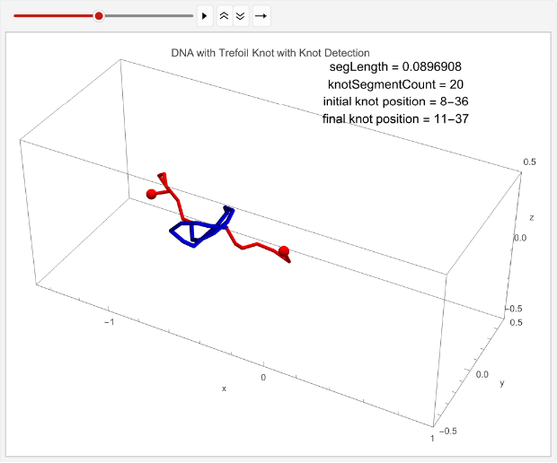
Animation:
animation=TableGraphics3D{Red,Sphere[p1,0.03],Sphere[p2,0.03],Tube[coords[[t]],0.01],Blue,Tube[knotColoring[t]]},,{t,timesteps};ListAnimate[animation,DefaultDuration->5]
Out[]=
Further Model Validation
Further Model Validation
One of the main objectives of this project has now been met: creating a model of a knot randomly moving along a chain of DNA segments and determining its displacement. The next objective is to collect data on the knot’s movement. In addition, by collecting data, we can ensure the model works properly across different environments.
Average Left-Hand Trefoil Displacement
Average Left-Hand Trefoil Displacement
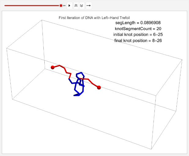
First, we will test the average displacement of 100 left-handed trefoil knots to determine if a trefoil knot has a pattern to its movement.
Displacement of 100 left-handed trefoil knots under the same parameters. Note that the number of iterations is modified to 1 to speed up runtime, but the full dataset was gathered on 100 iterations:
leftHandDisplaceStats=TablelinPositions=startPositions;knotEndpoints={};overall=overallGetSegments[];initialStart=overall[[1]];initialEnd=overall[[2]];If[i==1,coords=Join[{linPositions},Table[overall=overallGetSegments[];start=overall[[1]];end=overall[[2]];AppendTo[knotEndpoints,{initialStart,initialEnd}];Join[{p1},Table[getCoord[i],{i,2,n-1}],{p2}],{t,2,timesteps}]];,coords=Join[{linPositions},Table[Join[{p1},Table[getCoord[i],{i,2,n-1}],{p2}],{t,2,timesteps}]]];overall=overallGetSegments[];finalStart=overall[[1]];finalEnd=overall[[2]];AppendTo[knotEndpoints,{finalStart,finalEnd}];Ifi==1,animation=TableGraphics3D{Red,Sphere[p1,0.03],Sphere[p2,0.03],Tube[coords[[t]],0.01],Blue,Tube[knotColoring[t]]},,{t,timesteps};Print[ListAnimate[animation,DefaultDuration->5]];finalStart-initialStart,{i,1,1};
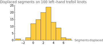
While the positions of 100 knots were collected, some of these positions might not have been valid. That is, they might have returned Nulls. This is because the knots moved towards the DNA chain’s fixed endpoints, eventually slipping off and untying themselves. While interesting, these Nulls are not important to our study of knot displacement and thus must be removed.
Cleaning the data of Nulls:
intLeftHandDisplaceStats=Select[leftHandDisplaceStats,NumericQ];HistogramintLeftHandDisplaceStats,
Out[]=
Calculating the mean knot displacement:
N[Mean[intLeftHandDisplaceStats]]
Out[]=
2.40404
The average displacement of a left-hand trefoil knot across 100 runs is 2.404 segments, meaning a left-handed trefoil tends to travel 2.404 segments to the right over 200 timesteps. However, this naturally brings up the question of whether the knot’s left-handedness impacts the direction it moves. Thus, we re-modeled the knot and created a right-handed trefoil instead.
Average Right-Hand Trefoil Displacement
Average Right-Hand Trefoil Displacement
Making a Right-Hand Trefoil
Making a Right-Hand Trefoil
Function to make a right-handed trefoil knot and scale it for constant segment length:
In[]:=
makeRightHandTrefoilKnot[knotSegmentCount_]:=Module[{steps,rawPoints,segments,unitVectors},steps=Subdivide[-Pi/8,(49Pi)/32,knotSegmentCount];rawPoints=Table[{Sin[t]+2Sin[2t],Cos[t]-2Cos[2t],Sin[3t]},{t,steps}];segments=Partition[rawPoints,2,1];unitVectors=Map[segLength*Normalize[#[[2]]-#[[1]]]&,Most[segments]];FoldList[Plus,rawPoints[[1]],unitVectors]]
Function to remake linPositions with the tails and the knot in the proper place after translation/rotation:
In[]:=
makeLinPos[point1_,point2_,n_,vert_,knotSegmentCount_,knotPoints_]:=Module[{preEndIndex,postStartIndex,ogPointDist,prePoints,startAnchor,endAnchor,knotVec,targetVec,axis,angle,rotation,rotatedKnot,translatedKnot,postPoints,linPositions},ogPointDist=Norm[p2-p1]/(n-1);preEndIndex=Floor[(n-knotSegmentCount)/2-1];postStartIndex=Floor[(n+knotSegmentCount)/2+1];prePoints=Table[point1+(i/(n-1))*(point2-point1)+{0,If[EvenQ[i],vert,-vert],0},{i,0,preEndIndex+1}];startAnchor=prePoints[[-1]];endAnchor=startAnchor+(knotSegmentCount/(n-1))*(p2-p1);knotVec=knotPoints[[-1]]-knotPoints[[1]];targetVec=endAnchor-startAnchor;axis=Cross[knotVec,targetVec];angle=VectorAngle[knotVec,targetVec];rotation=If[Norm[axis]==0,Identity,RotationTransform[angle,axis]];rotatedKnot=Map[rotation,knotPoints];translatedKnot=Map[#+(startAnchor-rotatedKnot[[1]])&,rotatedKnot];postPoints=Table[translatedKnot[[-1]]+(i/(n-1))*(point2-point1)+{0,If[EvenQ[i],vert,-vert],0},{i,0,n-postStartIndex+1}];postPoints[[1]]=translatedKnot[[-1]];linPositions=Join[Most[prePoints],Most[translatedKnot],postPoints];p2=linPositions[[-1]];linPositions]
Re-defining initial parameters for a right-hand trefoil:
In[]:=
n=30;knotSegmentCount=20;p1={-1,0,0};p2={1,0,0};vert=0.05;dist=Norm[p2-p1];tempLength=dist/n;segLength=Sqrt[tempLength^2+vert^2];
Creating the proper coordinates for a right-handed trefoil and its tails:
knotPoints=makeRightHandTrefoilKnot[knotSegmentCount];linPositions=makeLinPos[p1,p2,n,vert,knotSegmentCount,knotPoints];startPositions=linPositions;Graphics3D[Tube[linPositions]]
Out[]=

Collecting Data
Collecting Data
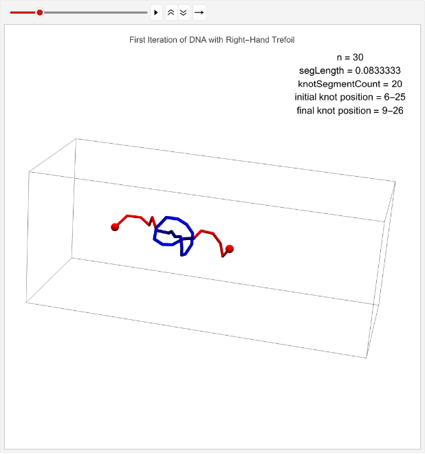
Now that we’ve created a right-hand trefoil, we can simulate it across 100 simulations to determine if it has a tendency to its movements.
Collecting data on the average displacement of a right-hand trefoil across 100 simulations. Note that the number of iterations is modified to 1 to speed up runtime, but the full dataset was gathered on 100 iterations:
rightHandDisplaceStats=TablelinPositions=startPositions;knotEndpoints={};overall=overallGetSegments[];initialStart=overall[[1]];initialEnd=overall[[2]];If[i==1,coords=Join[{linPositions},Table[overall=overallGetSegments[];start=overall[[1]];end=overall[[2]];AppendTo[knotEndpoints,{initialStart,initialEnd}];Join[{p1},Table[getCoord[i],{i,2,n-1}],{p2}],{t,2,timesteps}]];,coords=Join[{linPositions},Table[Join[{p1},Table[getCoord[i],{i,2,n-1}],{p2}],{t,2,timesteps}]]];overall=overallGetSegments[];finalStart=overall[[1]];finalEnd=overall[[2]];AppendTo[knotEndpoints,{finalStart,finalEnd}];Ifi==1,animation=TableGraphics3D{Red,Sphere[p1,0.03],Sphere[p2,0.03],Tube[coords[[t]],0.01],Blue,Tube[knotColoring[t]]},,{t,timesteps};Print[ListAnimate[animation,DefaultDuration->5]];finalStart-initialStart,{i,1,1};
Cleaning the data of Nulls where the knot reached the end:
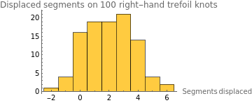
intRightHandDisplaceStats=Select[rightHandDisplaceStats,NumericQ];HistogramintRightHandDisplaceStats,
Out[]=
Finding the average knot displacement:
N[Mean[intRightHandDisplaceStats]]
Out[]=
2.02
The mean displacement of a right-handed trefoil was 2.02 DNA segments. Clearly, there is not an obvious difference in displacement based on a trefoil knot’s chirality, or at most, a slight reduction in displacement for a right-handed trefoil. More generally, a trefoil knot seems to travel about 2 segments to the right in this simulation. This may be because of the method of modeling random motion, where each segment’s point is randomly chosen from the left to right. Another interesting thing to note is the fact that both histograms of the trefoil knots show a surprisingly symmetrical, mound-shaped distribution of knot displacement. This could be due to the RandomReal used in random point selection, which may model a normal distribution.
Average Trefoil Knot Size Difference
Average Trefoil Knot Size Difference
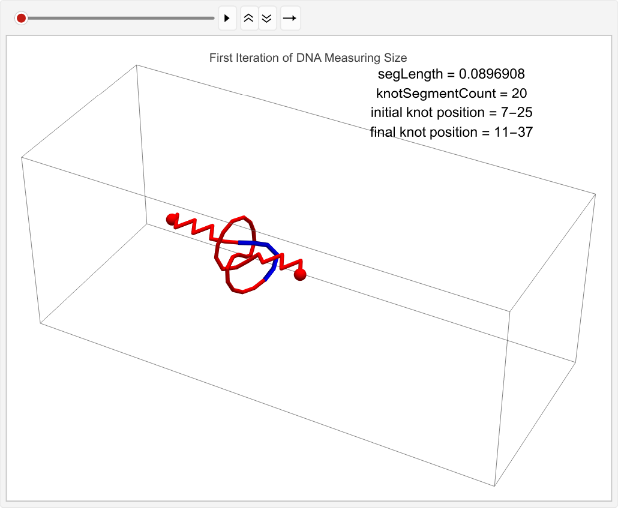
Next, we want to study the average size difference between the knot at the start of the animation versus the end of it. For our purposes, we will define size as the number of segments between the first and last crossing of the knot. We will then take the average size difference across 100 knots to determine any patterns in knot size.
Determining the size of a trefoil knot along the chain across 100 runs. Note that the number of iterations is modified to 1 to speed up runtime, but the full dataset was gathered on 100 iterations::
In[]:=
sizeStats=QuietTabletimesteps=400;knotEndpoints={};linPositions=startPositions;overall=overallGetSegments[];initialStart=overall[[1]];initialEnd=overall[[2]];initialSize=Abs[initialEnd-initialStart];If[i==1,coords=Join[{linPositions},Table[overall=overallGetSegments[];start=overall[[1]];end=overall[[2]];AppendTo[knotEndpoints,{initialStart,initialEnd}];Join[{p1},Table[getCoord[i],{i,2,n-1}],{p2}],{t,2,timesteps}]];,coords=Join[{linPositions},Table[Join[{p1},Table[getCoord[i],{i,2,n-1}],{p2}],{t,2,timesteps}]]];overall=overallGetSegments[];finalStart=overall[[1]];finalEnd=overall[[2]];AppendTo[knotEndpoints,{finalStart,finalEnd}];finalSize=Abs[finalEnd-finalStart];Ifi==1,animation=TableGraphics3D{Red,Sphere[p1,0.03],Sphere[p2,0.03],Tube[coords[[t]],0.01],Blue,Tube[knotColoring[t]]},,{t,timesteps};Print[ListAnimate[animation,DefaultDuration->5,AnimationRunning->False]];{initialSize,finalSize},{i,1,1};
Cleaning sizeStats of Nulls from knots reaching the end:
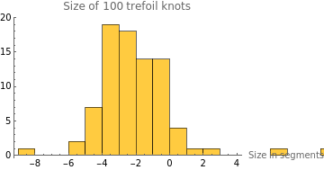
intSizeStats=Select[sizeStats,VectorQ[#,NumericQ]&];sizeDiff=Table[intSizeStats[[i]][[2]]-intSizeStats[[i]][[1]],{i,1,Length[intSizeStats]}];HistogramsizeDiff,
Out[]=
Determining the mean size difference:
N[Mean[sizeDiff]]
Out[]=
-2.65476
The average size difference in each knot after 400 frames is roughly -2.65 segments. Across 100 trefoil knots, it seems that through random motion, trefoil knots tend to shrink in size by 2.65 segments on average. This statistic’s parameter seems to be slightly more right-skewed than the histogram of knot displacement, which shows that trefoil knots tend to decrease in size rather than increase.
Increasing N on Average Knot Displacement
Increasing N on Average Knot Displacement
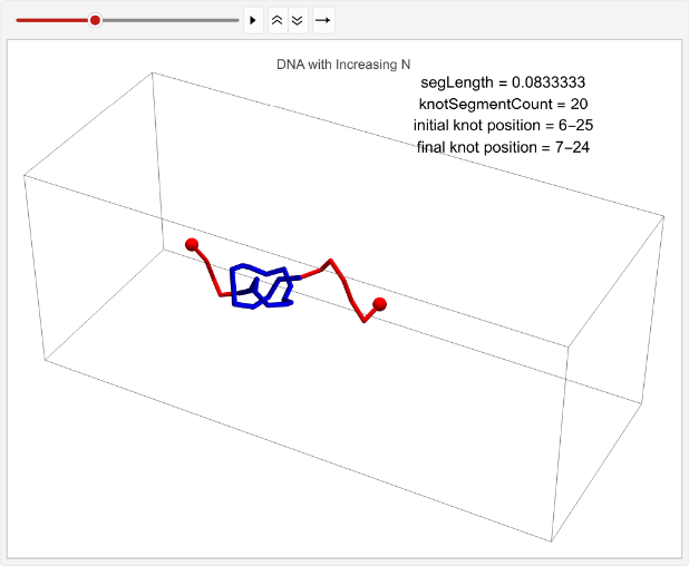
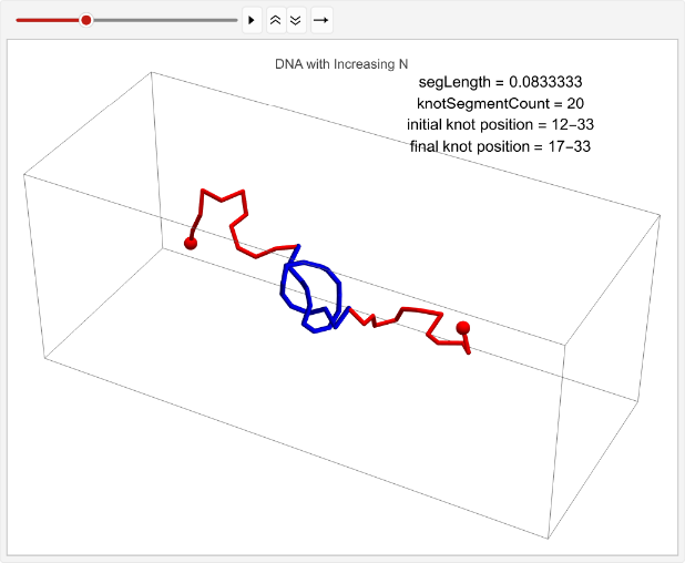
Next, we can impose parameters onto our model to determine their effect. For example, we can increase the number of chain segments (n) and measure the corresponding knot displacement. By doing so, we can find a correlation relating DNA length and knot movement.
Determining the effect of increasing n on knot displacement. Note that the number of iterations is modified to 2 to speed up runtime, but the full dataset was gathered on 15 iterations:
vert=0.05;n=30;timesteps=100;knotSegmentCount=20;incNStats=Tablen++;linPositions=makeLinPos[{-1,0,0},{1,0,0},n,vert,knotSegmentCount,knotPoints];knotEndpoints={};overall=overallGetSegments[];initialStart=overall[[1]];initialEnd=overall[[2]];If[i==1||i==15,coords=Join[{linPositions},Table[overall=overallGetSegments[];start=overall[[1]];end=overall[[2]];AppendTo[knotEndpoints,{initialStart,initialEnd}];Join[{p1},Table[getCoord[i],{i,2,n-1}],{p2}],{t,2,timesteps}]];,coords=Join[{linPositions},Table[Join[{p1},Table[getCoord[i],{i,2,n-1}],{p2}],{t,2,timesteps}]]];overall=overallGetSegments[];finalStart=overall[[1]];finalEnd=overall[[2]];AppendTo[knotEndpoints,{finalStart,finalEnd}];Ifi==1||i==15,animation=TableGraphics3D{Red,Sphere[p1,0.03],Sphere[p2,0.03],Tube[coords[[t]],0.01],Blue,Tube[knotColoring[t]]},,{t,timesteps};Print[ListAnimate[animation,DefaultDuration->5]];{n,finalStart-initialStart},{i,1,2};
Graphing the absolute displacement against n:
intIncNStats=Select[incNStats,VectorQ[#,NumericQ]&];absIncNStats=Abs[intIncNStats];eqN=Fit[absIncNStats,{1,x},x];incNCoeff=N[Correlation[Table[absIncNStats[[i]][[1]],{i,1,Length[absIncNStats]}],Table[absIncNStats[[i]][[2]],{i,1,Length[absIncNStats]}]]];ShowListPlot[absIncNStats,PlotStyle->Blue],Plot[eqN,{x,1,50}],
Out[]=
From the graph and the line of best fit, there is a moderate positive correlation (r=0.496) between the number of segments in the chain and the absolute displacement of the knot. This is likely because more segments allow for more motion in the DNA chain, displacing the knot further. However, because this sample size was only 15 knots due to constraints in the collisions’ computational ability, the true correlation may differ.
Increasing Knot Segment Count on Average Knot Displacement
Increasing Knot Segment Count on Average Knot Displacement
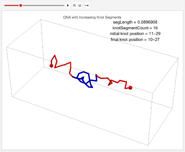
Next, we want to increase the number of knot segments rather than the number of total chain segments. We can compare the correlation and trends of the knot’s displacement between increasing knot segments versus increasing chain segments.
Gathering data on the effect of increasing the number of knot segments on knot displacement. Note that the number of iterations is modified to 2 to speed up runtime, but the full dataset was gathered on 15 iterations:
vert=0.05;n=40;knotSegmentCount=15;incKnotStats=TableknotSegmentCount++;knotPoints=makeRightHandTrefoilKnot[knotSegmentCount];linPositions=makeLinPos[{-1,0,0},{1,0,0},n,vert,knotSegmentCount,knotPoints];knotEndpoints={};overall=overallGetSegments[];initialStart=overall[[1]];initialEnd=overall[[2]];If[i==1||i==15,coords=Join[{linPositions},Table[overall=overallGetSegments[];start=overall[[1]];end=overall[[2]];AppendTo[knotEndpoints,{initialStart,initialEnd}];Join[{p1},Table[getCoord[i],{i,2,n-1}],{p2}],{t,2,timesteps}]];,coords=Join[{linPositions},Table[Join[{p1},Table[getCoord[i],{i,2,n-1}],{p2}],{t,2,timesteps}]]];overall=overallGetSegments[];finalStart=overall[[1]];finalEnd=overall[[2]];AppendTo[knotEndpoints,{finalStart,finalEnd}];Ifi==1||i==15,animation=TableGraphics3D{Red,Sphere[p1,0.03],Sphere[p2,0.03],Tube[coords[[t]],0.01],Blue,Tube[knotColoring[t]]},,{t,timesteps};Print[ListAnimate[animation,DefaultDuration->5]];{knotSegmentCount,finalStart-initialStart},{i,1,2};
Cleaning incKnotStats of Nulls:
In[]:=
intIncKnotStats=Select[incKnotStats,VectorQ[#,NumericQ]&];absIncKnotStats=Abs[intIncKnotStats];
Graphing knot displacement vs. knot segment count:
eqKnot=Fit[absIncKnotStats,{1,x},x];incKnotCoeff=N[Correlation[Table[absIncKnotStats[[i]][[1]],{i,1,Length[absIncKnotStats]}],Table[absIncKnotStats[[i]][[2]],{i,1,Length[absIncKnotStats]}]]];ShowListPlot[absIncKnotStats,PlotStyle->Blue],Plot[eqKnot,{x,1,50}],
Out[]=
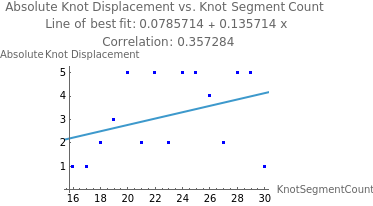
The correlation between the number of segments in the knot and its displacement is moderate, with a Pearson correlation coefficient of 0.357. This is less than the earlier correlation coefficient between the number of segments in the total chain and the knot’s displacement (0.496). This is likely because, as knot size increases, the tails’ size similarly decrease, reducing the amount of distance the knot as a whole can move. However, if the knot size and n size proportionally increased, we might find a stronger correlation.
Increasing Both Chain Length and Knot Segment Count on Average Knot Displacement:
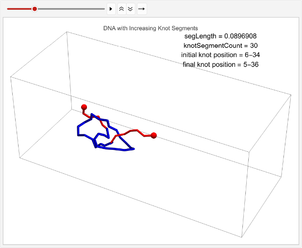
Increasing Both Chain Length and Knot Segment Count on Average Knot Displacement:
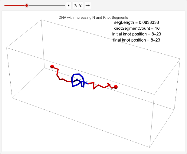
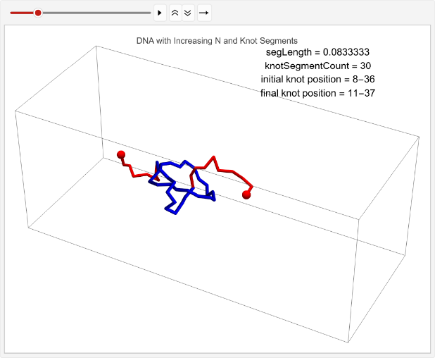
Determining knot displacement while increasing both the number of DNA chain segments and knot segments. Note that the number of iterations is modified to 2 to speed up runtime, but the full dataset was gathered on 15 iterations:
vert=0.05;n=30;knotSegmentCount=15;incRatioStats=TableknotSegmentCount++;n++;knotPoints=makeRightHandTrefoilKnot[knotSegmentCount];linPositions=makeLinPos[{-1,0,0},{1,0,0},n,vert,knotSegmentCount,knotPoints];knotEndpoints={};overall=overallGetSegments[];initialStart=overall[[1]];initialEnd=overall[[2]];If[i==1||i==15,coords=Join[{linPositions},Table[overall=overallGetSegments[];start=overall[[1]];end=overall[[2]];AppendTo[knotEndpoints,{initialStart,initialEnd}];Join[{p1},Table[getCoord[i],{i,2,n-1}],{p2}],{t,2,timesteps}]];,coords=Join[{linPositions},Table[Join[{p1},Table[getCoord[i],{i,2,n-1}],{p2}],{t,2,timesteps}]]];overall=overallGetSegments[];finalStart=overall[[1]];finalEnd=overall[[2]];AppendTo[knotEndpoints,{finalStart,finalEnd}];Ifi==1||i==15,animation=TableGraphics3D{Red,Sphere[p1,0.03],Sphere[p2,0.03],Tube[coords[[t]],0.01],Blue,Tube[knotColoring[t]]},,{t,timesteps};Print[ListAnimate[animation,DefaultDuration->5]];{knotSegmentCount/n,finalStart-initialStart},{i,1,2};
Cleaning the data of Nulls:
In[]:=
intIncRatioStats=Select[incRatioStats,VectorQ[#,NumericQ]&];absIncRatioStats=Abs[intIncRatioStats];
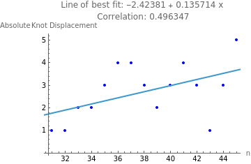
Graphing the knot displacement against the ratio of knotSegmentCount : n:
eqRatio=Fit[absIncRatioStats,{1,x},x];ratioCoeff=N[Correlation[Table[absIncRatioStats[[i]][[1]],{i,1,Length[absIncRatioStats]}],Table[absIncRatioStats[[i]][[2]],{i,1,Length[absIncRatioStats]}]]];Show[ListPlot[absIncRatioStats,PlotStyle->Blue],Plot[eqRatio,{x,0,1}],PlotLabel->StringJoin["Line of best fit: ",ToString[eqRatio],"\n Correlation: ",ToString[ratioCoeff]],AxesLabel->{"knotSegmentCount : n","Absolute Segment Displacement"}]
Out[]=
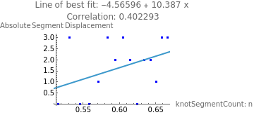
The correlation between the ratio of knotSegmentCount:n and absolute segment displacement is moderately strong with a Pearson correlation coefficient of 0.402. This is actually stronger than the correlation coefficient between knot segment count and absolute segment displacement (0.357), which supports that increasing both knot segment count and chain length proportionally is more influential to absolute segment displacement rather than just increasing knot segment count.
Knot Formation
Knot Formation
Another objective of this project was to simulate knot formation. To simulate knot formation, we must start with an empty chain of line segments randomly moving and model it over hundreds of timesteps. It is still very unlikely that a trefoil knot will form, as a loop would have to form near the ends and pull itself over the endpoint, all through random motion. Thus, this is just a preliminary investigation to how unlikely the formation of a trefoil is.
Setting up the parameters for a long chain of chromatin with fixed endpoints. Note that the timesteps are decreased to 200 to reduce runtime, but the full tests were done on 1000 timesteps:
p1={-1,0,0};p2={1,0,0};timesteps=200;vert=0.05;dist=Norm[p2-p1];tempLength=dist/n;segLength=Sqrt[tempLength^2+vert^2];minDistance=Floor[segLength,0.01];n=70;linPositions=Table[p1+(i/(n-1))*(ogPointDist)+{0,If[EvenQ[i],vert,-vert],0},{i,1,n}];Graphics3D[Tube[linPositions]]
Out[]=

Creating the coordinates over each frame:
In[]:=
coords=Join[{linPositions},Table[Join[{p1},Table[getCoord[i],{i,2,n-1}],{p2}],{t,2,timesteps}]];
Animation:
In[]:=
animation=Table[Rasterize@Graphics3D[{Red,Sphere[p1,0.03],Sphere[p2,0.03],Tube[coords[[t]],0.01]},{PlotRange{{-2,2},{-1,1},{-1,1}},BoxedTrue,ImageSize600}],{t,timesteps}];ListAnimate[animation,DefaultDuration->5,AnimationRunning->False]
Out[]=
After 1000 timesteps on a piece of chromatin 70 segments long, a trefoil knot did not form. Even after several iterations, a trefoil knot was not found, making its formation seem extremely unlikely or almost impossible. Although this particular objective was unsuccessful, we did discover useful limits to this model; after 70 segments with 1000 timesteps, the calculations for each collision and position begin to slow, making it difficult to simulate longer sequences.
Figure Eight Knots
Figure Eight Knots
While the trefoil knot is a commonly found knot in DNA, other knots like the figure eight knot are possible as well. The figure eight knot has an Alexander-Briggs notation of , signifying that it has four crossings. It is the only knot with four crossings and can be formed during replication and topoisomerase activity. Because the main focus of this project was the trefoil knot, less analysis was done on figure eight knots. However, this section shows that a figure eight knot can be similarly modeled and in the future, properly analyzed for displacement.
4
1
First, we re-modeled a figure eight knot along the chain of DNA segments.
Making a figure eight knot:
knotSegmentCount=30;steps=Subdivide[-1Pi/10,17Pi/8,knotSegmentCount];rawPoints=Table[{Sin[t]+t/6,2Sin[t]Cos[t],(Sin[3t]Sin[t/4])},{t,steps}];Graphics3D[Tube[rawPoints],PlotRange->All,Boxed->False]
Out[]=

Re-defining initial constants:
In[]:=
n=40;vert=0.05;timesteps=200;p1={-1,0,0};p2={1,0,0};dist=Norm[p2-p1];tempLength=dist/n;segLength=Sqrt[tempLength^2+vert^2];minDistance=Floor[segLength,0.01];
Re-scaling the figure eight knot to be the constant segment length:
segments=Partition[rawPoints,2,1];unitVectors=Map[segLength*Normalize[#[[2]]-#[[1]]]&,Most[segments]];knotPoints=FoldList[Plus,rawPoints[[1]],unitVectors];Graphics3D[Tube[knotPoints]]
Out[]=

Creating the positions of the knot and its tails:
linPositions=makeLinPos[p1,p2,n,vert,knotSegmentCount,knotPoints];startPositions=linPositions;Graphics3D[Tube[linPositions],Axes->True]
Out[]=

Unlike a trefoil knot, the figure eight knot’s signature pattern in this knot code can take several forms, such as {U1, O2, O3, U4, O1, U2, O4, U3} and {U1, O2, U3, O4, U2, O1, U4, O3}, as well as their complements. These two sequences were used and can catch most figure eight knots in this model. However, further work should be done to identify more sequences.
Function for checking the pattern for a figure eight knot:
In[]:=
checkFigureEight[label_]:=Module[{pts},pts={};pts=Cases[{label},s:{___,u1_String,___,o2_String,___,o3_String,___,u4_String,___,o1_String,___,u2_String,___,o4_String,___,u3_String,___}/;StringMatchQ[u1,"U"~~__]&&StringMatchQ[o2,"O"~~__]&&StringMatchQ[o3,"O"~~__]&&StringMatchQ[u4,"U"~~__]&&StringMatchQ[o1,"O"~~__]&&StringMatchQ[u2,"U"~~__]&&StringMatchQ[o4,"O"~~__]&&StringMatchQ[u3,"U"~~__]&&StringDrop[o1,1]===StringDrop[u1,1]&&StringDrop[u2,1]===StringDrop[o2,1]&&StringDrop[o3,1]===StringDrop[u3,1]&&StringDrop[u4,1]===StringDrop[o4,1]:>{o1,u3}];If[pts=={},pts=Cases[{label},s:{___,o1_String,___,u2_String,___,u3_String,___,o4_String,___,u1_String,___,o2_String,___,u4_String,___,o3_String,___}/;StringMatchQ[o1,"O"~~__]&&StringMatchQ[u2,"U"~~__]&&StringMatchQ[u3,"U"~~__]&&StringMatchQ[o4,"O"~~__]&&StringMatchQ[u1,"U"~~__]&&StringMatchQ[o2,"O"~~__]&&StringMatchQ[u4,"U"~~__]&&StringMatchQ[o3,"O"~~__]&&StringDrop[o1,1]===StringDrop[u1,1]&&StringDrop[u2,1]===StringDrop[o2,1]&&StringDrop[o3,1]===StringDrop[u3,1]&&StringDrop[u4,1]===StringDrop[o4,1]:>{o1,u3}]];If[pts=={},pts=Cases[{label},s:{___,u1_String,___,o2_String,___,u3_String,___,o4_String,___,u2_String,___,o1_String,___,u4_String,___,o3_String,___}/;StringMatchQ[u1,"U"~~__]&&StringMatchQ[o2,"O"~~__]&&StringMatchQ[u3,"U"~~__]&&StringMatchQ[o4,"O"~~__]&&StringMatchQ[u2,"U"~~__]&&StringMatchQ[o1,"O"~~__]&&StringMatchQ[u4,"U"~~__]&&StringMatchQ[o3,"O"~~__]&&StringDrop[u1,1]===StringDrop[o1,1]&&StringDrop[o2,1]===StringDrop[u2,1]&&StringDrop[u3,1]===StringDrop[o3,1]&&StringDrop[o4,1]===StringDrop[u4,1]:>{u1,o3}]];If[pts=={},pts=Cases[{label},s:{___,o1_String,___,u2_String,___,o3_String,___,u4_String,___,o2_String,___,u1_String,___,o4_String,___,u3_String,___}/;StringMatchQ[o1,"O"~~__]&&StringMatchQ[u2,"U"~~__]&&StringMatchQ[o3,"O"~~__]&&StringMatchQ[u4,"U"~~__]&&StringMatchQ[o2,"O"~~__]&&StringMatchQ[u1,"U"~~__]&&StringMatchQ[o4,"O"~~__]&&StringMatchQ[u3,"U"~~__]&&StringDrop[o1,1]===StringDrop[u1,1]&&StringDrop[u2,1]===StringDrop[o2,1]&&StringDrop[o3,1]===StringDrop[u3,1]&&StringDrop[u4,1]===StringDrop[o4,1]:>{o1,u3}]];pts];
Re-defining a function for checking a figure eight pattern on a specified plane:
In[]:=
checkingSegDimensions[str_]:=Module[{label,crossingLabelsBySegment},label=getLabel[str][[1]];crossingLabelsBySegment=getLabel[str][[2]];label=checkLoops[label];pts=checkFigureEight[label];{pts,crossingLabelsBySegment}];
Determining the initial and final knot’s start points, and creating the frames for animation:
overall=overallGetSegments[];initialStart=overall[[1]];initialEnd=overall[[2]];coords=Join[{linPositions},Table[Join[{p1},Table[getCoord[i],{i,2,n-1}],{p2}],{t,2,timesteps}]];overall=overallGetSegments[];finalStart=overall[[1]];finalEnd=overall[[2]];Print["Figure eight knot moved from: ",initialStart,"-",finalStart]
Figure eight knot from: 8-10
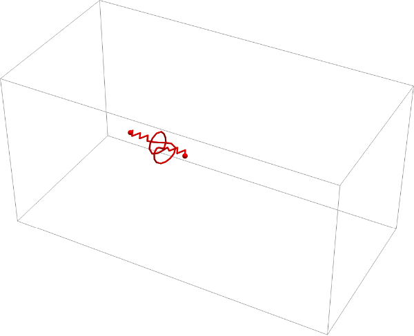
Animation:
animation=TableGraphics3D{Red,Sphere[p1,0.03],Sphere[p2,0.03],Tube[coords[[t]],0.01]},,{t,timesteps};ListAnimate[animation,DefaultDuration->5]
Out[]=

Conclusion
Conclusion
By using various collision detectors and projections, this project created a model of a knot traveling along a randomly moving strand of chromatin. With this model’s method of random movement, we concluded that both a left-handed and right-handed trefoil travel an average of 2 segments to the right and tend to shrink 2.65 segments in size. We also found that proportionally increasing both the number of segments in the knot and the number of segments in the chain has a moderate influence on knot displacement. Thus, we met our first objectives of modeling DNA movement and studying its tendencies. However, we did not detect knot formation in a chain of chromatin without a knot. This was mostly due to issues with function complexity, as the latency period to model larger chains increased quickly. Regardless, we inferred that knot formation was very unlikely in our model. Finally, we went one step further and modeled a figure eight knot’s movement along the chain, showing that this method of modeling DNA knots is applicable to other types of knots. Therefore, this project successfully modeled different knots along randomly moving chains of DNA line segments, as well as analyzing their motion and size.
Future Directions
Future Directions
For the future, the most immediate concern is using a more mathematically rigorous way to identify knots. Given more time, we could use Alexander polynomials, or continue to use this method of labelling crossings with more sequences analyzed and removed for unknot characteristics. Similarly, our collision detection could be improved to reduce the minimal collision distance. Yet more generally, this work could be expanded on by modeling knot formation or unknotting methods that could be used by topoisomerase II and IV. By continuing to study knot formation and movement, we can further understand mechanisms of replication and DNA damage for future applications like apoptosis-inducing medications.
Acknowledgements
Acknowledgements
I would like to thank my mentor, Dr. Dave DeBrota, for his constant guidance and support, particularly for the DNA random motion and knot identification. I would also like to thank William Choi-Kim and the other teaching assistants for their incredible help with creating knot sequences and exploring other invariants. Finally, I’d like to thank all the people who made this program enjoyable, like my teaching assistants and mentor groups.
References
References
◼
Deibler, R. W., Mann, J. K., Sumners, D. W. L., & Zechiedrich, L. (2007). Hin-mediated DNA Knotting and Recombining Promote Replicon Dysfunction and Mutation. BMC Molecular Biology, 8(1). https://doi.org/10.1186/1471-2199-8-44
◼
Ferréol, R. (2020). Figure-eight Knot. Mathcurve.com; Robert Ferréol. https://mathcurve.com/courbes3d.gb/noeuds/noeudenhuit.shtml
◼
george2079. (2014, April 1). Distance between Two Line Segments in 3-space. Mathematica and Wolfram Language Stack Exchange. https://mathematica.stackexchange.com/questions/45265/distance-between-two-line-segments-in-3-space
◼
Stauch, T., & Dreuw, A. (2016). Knots “Choke Off” Polymers upon Stretching. Angewandte Chemie (International Ed. In English), 55(2), 811–814. https://doi.org/10.1002/anie.201508706
CITE THIS NOTEBOOK
CITE THIS NOTEBOOK
Modeling DNA knot dynamics
by Sarah Park
Wolfram Community, STAFF PICKS, July 10, 2025
https://community.wolfram.com/groups/-/m/t/3499455
by Sarah Park
Wolfram Community, STAFF PICKS, July 10, 2025
https://community.wolfram.com/groups/-/m/t/3499455