ORIGINAL ARTICLE: Mulligan, Casey B., The Value of Pharmacy Benefit Management (2022). University of Chicago, Becker Friedman Institute for Economics Working Paper No. 2022-93, Available at SSRN: http://dx.doi.org/10.2139/ssrn.4163025
Article Abstract: In theory, equilibrium profits for drug patent holders would not involve significant restraints on production and patient utilization if the market had a mechanism for two-part pricing (Oi 1971) or quantity commitments (Murphy, Snyder, and Topel 2014). In fact, patent expiration has little effect on drug utilization especially when those drugs are delivered through insurance plans. This paper provides a quantitative model consistent with the theory and evidence in which pharmacy benefit management on behalf of insurance plans serves these and other purposes in both monopoly and oligopoly provider settings. Calibrating the model to the U.S. market, I conclude that pharmacy benefit management is worth at least $145 billion annually beyond its resource costs. PBM services add at least $192 billion annually in value to society compared to a manufacturer price-control regime. Requiring all PBM services to be self-provided by plan sponsors would forgo about 40 percent of the net value of PBM services largely by increasing management costs. Due to changes in the incidence of PBM services over the drug life cycle, the services encourage innovation even though they reduce the profits of incumbent manufacturers.
Model description
Model description
In this model, the marginal cost of the drug is normalized to one. Consumers have preferences over the quantity of a manufacturer’s drug and the quantity of sales by competitors, where and are symmetric substitutes. With no income
effects, demand functions that are linear in prices, and efficient quantities that are (a normalization of quantity units), the preferences must be those described by (up to the quasilinear term in expenditure on goods other than and ):
q
Q
q
Q
effects, demand functions that are linear in prices, and efficient quantities that are
q=Q=1
q
Q
u(q,Q)=
1
η
(q+Q)(η-1)ϵ+(η+ϵ)qQ-ϵ+
2
q
2
Q
2
η+ϵ
η-2ϵ
1+ϵ
where the constants and satisfy and . If consumers are allowed to purchase any amount of and at prices and , respectively, their demand functions are:
η
ϵ
ϵ<η<0
ϵ<-1
q
Q
p
P
q=≡D(p,P)
(ϵ+1)[ϵp+(η-ϵ)P]+(1-η)ϵ
η+ϵ
and the symmetric demand function for .
Q=D(P,p)
Setup and definitions
Setup and definitions
Economicreasoning.com is Casey Mulligan’s Wolfram Language package designed to infer user meaning from context, and to offer users push-button options for analysis. As a result, it can be used without user programming, and with just a minimal familiarity with the Wolfram language.
In[]:=
Get@"http://economicreasoning.com"
Proof & Logic Tools 6.4
(c) Copyright 2016, 2017, 2018, 2019, 2020, 2021, 2022 by JMJ Economics
Type for a list of commands in the package.
| ||||
In[]:=
u[q_,Q_]:=
1
η
(q+Q)ϵ(η-1)+qQ(η-ϵ)-ϵ+
2
q
2
Q
2
ϵ+η
η-2ϵ
1+ϵ
In[]:=
d[p_,P_]:=
(ϵ+1)(ϵp+(η-ϵ)P)+ϵ(1-η)
ϵ+η
In[]:=
SignConditions={ϵ<η<0,ϵ<-1};
In[]:=
c[avggap_]:=c0
2
(avggap)
rcalib=ϵ-,η-,r,β1+Max0,-(*midpointofpartiallyidentifiedset.Thelowerbbdofβmakes==discr*),β20;
1+5
5
1
2
3
10
1
2
ϵ+4rϵ+8r+η-4rη
2
ϵ
ϵ+η
2
linterm
In[]:=
p0=;
ϵ
ϵ+1
Solution guesses
Solution guesses
In[]:=
eqm[q,c0_]:=ϵ
c0(ϵ+η)-2(ϵ+1)η
c0-2(ϵ+1)ηϵ
2
(ϵ+η)
In[]:=
eqm[L,c0_]:=
1
ϵ+1
c0ϵ-(ϵ+1)η(ϵ+2-η)
2
(ϵ+η)
2
ϵ
c0-2(ϵ+1)ηϵ
2
(ϵ+η)
In[]:=
eqm[m,c0_]=[eqm[q,c0],eqm[q,c0]]//Simplify
(1,0)
u
Out[]=
ϵ(-2η+c0)
2
(1+ϵ)
2
(ϵ+η)
(1+ϵ)(-2ϵ(1+ϵ)η+c0)
2
(ϵ+η)
In[]:=
eqm[r,c0_]:=*
1
4
c0(ϵ+η)(4βϵ+3η-3βη)-2(1+ϵ)η((-1+3β)ϵ-2(-1+β)η)
c0ϵ-(1+ϵ)(ϵ+2-η)η
2
(ϵ+η)
2
ϵ
(1+ϵ)η(ϵ+η)
c0ϵ(ϵ+η)-(1+ϵ)η(ϵ+βϵ+η-βη)
In[]:=
eqm[r,c0_]:=-
(1+ϵ)η(ϵ+η)(2(1+β)ϵ(1+ϵ)η-c0(ϵ+η)(4βϵ+3η-3βη))
4ϵ(2(ϵ+2-η)+ϵ-c0(1+ϵ)η(4-+2ϵ+(1+6η)))
2
(1+ϵ)
2
ϵ
2
η
2
c0
3
(ϵ+η)
3
ϵ
2
η
2
η
2
ϵ
In[]:=
discr=+16+8rϵ(ϵ+η)(4+5η+ϵ(3-2η)η+3(-1+η)+(4-3η-4ϵ+3)+β(-2(-2+η)+3(1-2η)+ϵη(-7+6η)));
2
(ϵ+η)
2
(4βϵ+3η-3βη)
2
r
2
ϵ
2
((-1+β)+ϵ(-1+2η)+η(1+η-βη))
2
ϵ
3
ϵ
2
ϵ
2
η
2
β
3
ϵ
2
ϵ
2
η
3
η
2
ϵ
2
η
In[]:=
discr=+16+8rϵ(ϵ+η)(-4+8η-3+3ϵη(1+2η)+β(12+(4-8η)+3-ϵη(7+6η)));
2
(ϵ+η)
2
(4βϵ+3η-3βη)
2
r
2
ϵ
2
(η+ϵ(-1+2η))
3
ϵ
2
ϵ
2
η
3
ϵ
2
ϵ
2
η
In[]:=
linterm=(ϵ+η)(4βϵ+3η-3βη)+4rϵ(ϵ+(3+β)+2ϵη+η(-1+η-βη));
2
ϵ
In[]:=
linterm=(ϵ+η)(4βϵ+3η-3βη)+4rϵ(ϵ+4-η+2ϵη);
2
ϵ
In[]:=
denom=;
8r
2
ϵ
2
(ϵ+η)
η(ϵ+1)
In[]:=
inferredc0=;
linterm+Sqrt[discr]
denom
Monopoly
Monopoly
In[]:=
monopoly[L]=;
η+(2η-1)ϵ
2(ϵ+1)η
In[]:=
monopoly[q0]=;
2ϵ-η
2ϵ
In[]:=
monopoly[m,c0_]=;
1
2(1+ϵ)η
c0ϵ(+2ϵ+(-1+2η))-4(2ϵ-η)
2
η
2
η
2
ϵ
2
(1+ϵ)
2
η
c0ϵ(ϵ+η)-2(1+ϵ)(2ϵ-η)η
In[]:=
monopoly[q,c0_]=;
2ϵ-η
2ϵ
c0ϵ(ϵ+η)-4(1+ϵ)(2ϵ-η)η
c0ϵ(ϵ+η)-2(1+ϵ)(2ϵ-η)η
Results: Demand curve properties
Results: Demand curve properties
Near P = p = , the p-elasticity of q demand is ϵ < 0
ϵ
1+ϵ
In[]:=
FullSimplifypD[Log@d[p,P],p]==ϵ,p==P==
ϵ
1+ϵ
Out[]=
True
q demand gets less elastic with P (approaching 0), and more elastic with p (approaching ∞)
Increase both together makes q demand more elastic
In[]:=
pD[Log@d[p,P],p]//SimplifyFullSimplify[D[%,P]>0∧D[%,p]<0,p>0∧P>0∧And@@SignConditions]FullSimplify[D[%%,P]+D[%%,p]<0/.P->p,p>0∧P>0∧And@@SignConditions]
Out[]=
pϵ(1+ϵ)
ϵ-ϵη+(1+ϵ)(pϵ+P(-ϵ+η))
Out[]=
True
Out[]=
True
Results: Ex poste equilibrium
Results: Ex poste equilibrium
Confirm that d reflects consumer optimization
In[]:=
(1,0)
u
(0,1)
u
Out[]=
True
Bertrand reaction function
In[]:=
D[(p-1)d[p,P],p]==0/.p-P//Simplify
1
2
ϵ+η
ϵ+1
η-ϵ
ϵ
Out[]=
True
This reaction function, evaluated at P m, also describes ex ante equilibrium list price
Profit-maximization problem is concave
In[]:=
TheoryGuru[SignConditions,D[(p-1)d[p,P],p,p]<0]
Out[]=
True
Symmetric equilibrium
In[]:=
p==-P/.p|Pp0//Simplify
1
2
ϵ+η
ϵ+1
η-ϵ
ϵ
Out[]=
True
In[]:=
d[p0,p0]==//Simplify
ϵ
ϵ+η
Out[]=
True
Monopoly price (without quantity commitments)
In[]:=
TheoryGuru{SignConditions,pmonopoly[L],qmonopoly[q0],Q0},p[q,Q]>p0∧q+Q<2d[p0,p0]∧D[q,Q]-1q,q0∧D[q,Q]-1q,q,q<0
(1,0)
u
(1,0)
u
(1,0)
u
Out[]=
True
Equilibrium vs generic pricing
In[]:=
0-(p0-1)q
1
ϵ
(1+ϵ)(ϵ+η)
u[1,1]-2*1-(u[q,q]-2q)
2*1
ϵ
η
Out[]=
True
In[]:=
u[1,1]-2*1-(u[q,q]-2q)
2*1
η
2
1
ϵ+1
1
ϵ+η
Out[]=
True
In[]:=
1-p0q
1
ϵ+η+ϵη
(1+ϵ)(ϵ+η)
Out[]=
True
Results: Ex ante equilbrium
Results: Ex ante equilbrium
Full marginal cost of q
In[]:=
ThreadGraduff[dmd[m,M],dmd[M,m]]-dmd[m,M]-dmd[M,m]-cff,{m,M}0//.[dmd[m,M],dmd[M,m]]m,[dmd[m,M],dmd[M,m]]M,Mm//SimplifyTheoryGuruindslope2D[dmd[m,m],m]<0,(l+L-2m)>0,%,1<m1+(l+L-2m)
L-M+l-m
2
(1,0)
uff
(0,1)
uff
′
cff
1
2
′
cff
1
2
-indslope
Out[]=
(l+L-2m)+2(-1+m)[m,m]+[m,m]0,(l+L-2m)+2(-1+m)[m,m]+[m,m]0
′
cff
1
2
(0,1)
dmd
(1,0)
dmd
′
cff
1
2
(0,1)
dmd
(1,0)
dmd
Out[]=
True
For monopolist
In[]:=
TheoryGuruDtuff[q,0]-q-cff,q0,Dtm==[q,0],q,Dt[l,q]==-0,m==[q,0],indslope==<0,(l-m)>0,1<m1+(l-m)1-[q,0](l-m)
l-m
2
(1,0)
uff
(1,0)
uff
1
D[q,0],q
(1,0)
uff
′
cff
1
2
1
2
′
cff
1
2
-indslope
1
2
(2,0)
uff
′
cff
1
2
Out[]=
True
Consumer rationality
In[]:=
eqm[q,c0]==d[eqm[m,c0],eqm[m,c0]]//Simplify
Out[]=
True
MV full MC
In[]:=
eqm[m,c0]1+[eqm[L,c0]-eqm[m,c0]]//Simplify
′
c
-2D[d[m,m],m]
Out[]=
True
In[]:=
m1-[q,0]/.{L->monopoly[L],m->monopoly[m,c0]}//Simplify
1
2
(2,0)
u
′
c
L-m
2
Out[]=
True
Optimal list price
In[]:=
TheoryGuru[{SignConditions,L==eqm[L,c0],m==eqm[m,c0]},D[(L-1)d[L,m],L]==0∧D[(L-1)d[L,m],L,L]<0]
Out[]=
True
Equilibrium rebate rate
In[]:=
β
1-β
u[q,q]-2(1-r)Lq-c[L-m]-u[q0,Q0]-Lq0-(1-r)Lq-(Q0-q)m-c
L-m
2
((1-r)L-1)q-(L-1)q0
Out[]=
True
In[]:=
r==eqm[r,inferredc0]//Simplify
Out[]=
True
Properties
Properties
The equilibrium list price is between one (MC) and the list price resulting from ex poste competition
In[]:=
TheoryGuru[{SignConditions,L==eqm[L,c0],m==eqm[m,c0],c0>0},1<m<L<p0]
Out[]=
True
In[]:=
TheoryGuru{SignConditions,L==eqm[L,c0],m==eqm[m,c0],c0==0},[1,1]==1==m<L
(1,0)
u
Out[]=
True
not to the quantities q = Q = 1 that would be efficient without compliance costs.
In[]:=
TheoryGuru[{SignConditions,q==eqm[q,c0],c0>0},d[p0,p0]<q<1]
Out[]=
True
In[]:=
TheoryGuru[{SignConditions,m==eqm[m,c0],L==eqm[L,c0],q0==d[L,m],Q0==d[m,L],c0>0},q0<eqm[q,c0]<Q0∧q0<eqm[q,c0]<1]
Out[]=
True
In[]:=
TheoryGuru[{SignConditions,q==eqm[q,c0],c0==0},d[p0,p0]<q==1==d[1,1]]
Out[]=
True
Analytical results for monopoly
In[]:=
TheoryGuru[{SignConditions},0<monopoly[q0]<1<monopoly[L]]
Out[]=
True
In[]:=
TheoryGuru[{SignConditions,c0>0},monopoly[m,c0]>1]
Out[]=
True
Numerical results
Numerical results
In[]:=
rsolve={qo->eqm[q,inferredc0],mo->eqm[m,inferredc0],Lo->eqm[L,inferredc0],c0->inferredc0,qm->monopoly[q,c0],qm0->monopoly[q0]};
Ex ante vs ex poste: oligopoly
In[]:=
"","","","",,,,/.rsolve//.rcalib//N//Transpose//Grid
Qexante
Qexposte
Dprofit
rebate
Dsurplus
rebate
Listexante
Listexposte
eqm[q,inferredc0]
d[p0,p0]
((1-r)Lo-1)qo-(p0-1)d[p0,p0]
rLoqo
u[qo,qo]-2qo-c[Lo-mo]-(u[d[p0,p0],d[p0,p0]]-2d[p0,p0])
2rLoqo
Lo
p0
Out[]=
Qexante Qexposte | 1.34202 |
Dprofit rebate | -0.946418 |
Dsurplus rebate | 0.465288 |
Listexante Listexposte | 0.80049 |
Ex ante vs ex poste: monopoly
Monopolists gets all surplus
In[]:=
""," ",Grid@1,"","Ex poste ","",," ",Grid@1,1+,,//.rsolve//.rcalib//N//Transpose//Grid
Qexante
Qexposte
Revexante
Revexposte
Revolipoly
Revmonopoly
Exanteolipoly
Expostemonopoly
qm
qm0
u[qm,0]-c[monopoly[L]-monopoly[m,c0]]-u[qm0,0]
monopoly[L]qm0
p0d[p0,p0]
monopoly[L]monopoly[q0]
(1-r)Loqo
monopoly[L]monopoly[q0]
Out[]=
Qexante Qexposte | 1.91132 | ||||||||
|
|
Quantity levels
In[]:=
{{" ","No PBM","PBM"}}~Join~Transpose[{{"Early","Late","Generic"},{qm0,2d[p0,p0],2d[1,1]}/2(*noPBM*),{qm,2qo,2d[1,1]}/2(*PBM*)}//.rsolve//.rcalib//N]//Grid
Out[]=
No PBM | PBM | |
Early | 0.395833 | 0.756565 |
Late | 0.705882 | 0.947306 |
Generic | 1. | 1. |
Plots
Plots
In[]:=
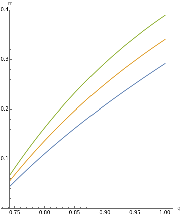
ParametricPlot[{eqm[q,c0],eqm[r,c0]}/.{{β->1/2},{β->3/4},{β->1}}/.rcalib//Evaluate,{c0,0,.6},AspectRatioFull,AxesLabel{"q","rr"},PlotRange{Automatic,{0,.4}}]
Out[]=
CITE THIS NOTEBOOK
CITE THIS NOTEBOOK
Quantitative market-equilibrium model of pharmaceutical markets with pharmacy benefit management
by Casey Mulligan
Wolfram Community, STAFF PICKS, February 22, 2024
https://community.wolfram.com/groups/-/m/t/3128728
by Casey Mulligan
Wolfram Community, STAFF PICKS, February 22, 2024
https://community.wolfram.com/groups/-/m/t/3128728