Questions and Comments
Questions and Comments
Session 1
Session 1
Questions from the session “Introduction to Variational Quantum Algorithms”.
Question from Yuliya Nesterova:
How to embed small circuits (a few gates) within larger circuits (built up of subcircuits) in the quantum framework? Thanks!
How to embed small circuits (a few gates) within larger circuits (built up of subcircuits) in the quantum framework? Thanks!
I assume you’re asking how to embed a QuantumCircuitOperator within another QuantumCircuitOperator. Here’s how you can define a subcircuit:
In[]:=
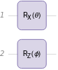
subcircuit=QuantumCircuitOperator[{"RX"[θ],"RZ"[ϕ]->{2}},"Parameters"->{θ,ϕ},"Label"->None];
In[]:=
subcircuit["Diagram",ImageSize->Tiny]
Out[]=
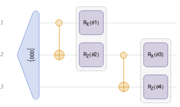
We can add it inside a QuantumCircuitOperator:
In[]:=
QuantumCircuitOperator[{"000","CNOT",subcircuit[θ1,θ2],"CNOT"->{2,3},subcircuit[θ3,θ4]->{2,3}}]["Diagram"]
Out[]=
If you already have a loaded circuit and need to insert subcircuits between specific gates:
In[]:=
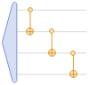
bigcircuit=QuantumCircuitOperator[{"0000","CNOT","CNOT"->{2,3},"CNOT"->{3,4}},"Label"->None]
Out[]=
QuantumCircuitOperator
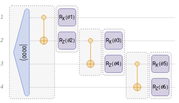
You can break it down into individual parts and construct a new circuit:
In[]:=
QuantumCircuitOperator[{bigcircuit[[;;2]],subcircuit[θ1,θ2],bigcircuit[[3]],subcircuit[θ3,θ4]->{2,3},bigcircuit[[4]],subcircuit[θ5,θ6]->{3,4}}]["Diagram"]
Out[]=
More detailed documentation here: https://resources.wolframcloud.com/PacletRepository/resources/Wolfram/QuantumFramework/ref/QuantumCircuitOperator.html
Question:If we have access to hpc (super computer) with mathematica can we push the number of qubits?
QuantumFramework is an abstract-level layer above Wolfram Language. Therefore, anything you can do in Wolfram Language to improve execution speed or optimize memory usage, such as parallel CPU/GPU programming, will also benefit QuantumFramework. You can check the documentation on parallel support at: https://reference.wolfram.com/language/CUDALink/tutorial/Overview.html
https://reference.wolfram.com/language/ParallelTools/tutorial/Overview.html
https://reference.wolfram.com/language/ParallelTools/tutorial/Overview.html
Question:
Is there big differences between Quantum Variational Algorithm and Quantum Annealing Algorithm in maintaining the state or manipulating them? Specifically of we are looking to the problem to minimize the energy can the cost function be an energy function?
Is there big differences between Quantum Variational Algorithm and Quantum Annealing Algorithm in maintaining the state or manipulating them? Specifically of we are looking to the problem to minimize the energy can the cost function be an energy function?
Yes, a common cost function for Variational Quantum Algorithms (VQAs) is the energy function, with the Variational Quantum Eigensolver (VQE) being a well-known example. Regarding state evolution, VQAs use discrete, parameterized quantum gates for unitary transformations, whereas Quantum Annealing (QA) relies on continuous-time evolution to maintain adiabaticity and remain in the ground state. If you’re interested in combinatorial optimization, a key application of QA, you may want to explore the Quantum Approximate Optimization Algorithm (QAOA), a VQA designed for such problems.
Session 2
Session 2
Questions from the session “Variational Quantum Eigensolver”:
Question about example:
How are the coordinates obtained ? Is it from experimental data already present or is it random ?
+
H3
How are the coordinates obtained ? Is it from experimental data already present or is it random ?
It’s from known parameters of the molecule, like for example chemical databases. In this particular case they were computed within the Hartree-Fock approximation using the GAMESS program (more information here: https://pennylane.ai/qml/demos/tutorial_mol_geo_opt).
Question about example:
What is the link between the dimension and the ansatz and cnot?
+
H3
What is the link between the dimension and the ansatz and cnot?
In this case, encoding the occupation numbers of the molecular spin-orbitals requires six qubits. The ansatz consists of alternating layers of Y-axis rotations (RY) and CNOT gates. The RY rotations allow each qubit to explore different quantum states—imagine a single qubit on the Bloch Sphere, where these rotations enable various pathways to reach a solution across its surface. Meanwhile, the CNOT gates serve as a fundamental mechanism for introducing interactions between the system’s elements.
We can represent it visually as follows:
In[]:=
ρ=QuantumCircuitOperator[{"RY"[α1]->{1},"RY"[α2]->{2},"RY"[α3]->{3},"CNOT"->{1,2},"CNOT"->{2,3}},"Parameters"->{α1,α2,α3}][];//FullSimplify
Here, we perform a test using qubit 1:
ρ1=FullSimplify@QuantumPartialTrace[ρ,{2,3}]
In[]:=
surface=ρ1["BlochVector"]//ComplexExpand
Out[]=
2CosSinSin[α2],0,-
α1
2
α1
2
2
Cos
α1
2
2
Sin
α1
2
In[]:=
ListPointPlot3D[Flatten[Table[surface,{α1,0,2π,.1},{α2,0,2π,.1},{α3,0,2π,.1}],1],BoxRatios->{1,1,1}]
Out[]=

Comment from David Fernando Ortega Tamayo:
Maybe we should try to connect with a real Quantum Computing like IBM, or AWS.
Maybe we should try to connect with a real Quantum Computing like IBM, or AWS.
You can find more about our connection to different QPU’s in the following documentation:
https://resources.wolframcloud.com/PacletRepository/resources/Wolfram/QuantumFramework/tutorial/QPUServiceConnect.html
https://resources.wolframcloud.com/PacletRepository/resources/Wolfram/QuantumFramework/tutorial/QPUServiceConnect.html
Session 3
Session 3
Questions from the session “Quantum Natural Gradient Descent”:
Question/Comment from Robert Lyons:
It would be good to supply a list of the names, their descriptions, and kinds of circuit elements used in quantum computing. I was not familiar with R, Z, CNOT, etc. gates. During my research into this subject, I came across such a list, and it took quite a bit of the mystery out of the material we’re studying in this class. My work in quantum mechanics was centered on semiconductor physics, not quantum computing. Thanks!
It would be good to supply a list of the names, their descriptions, and kinds of circuit elements used in quantum computing. I was not familiar with R, Z, CNOT, etc. gates. During my research into this subject, I came across such a list, and it took quite a bit of the mystery out of the material we’re studying in this class. My work in quantum mechanics was centered on semiconductor physics, not quantum computing. Thanks!
In the “Details and Options” section from QuantumOperator and QuantumCircuitOperator you can find the list of gates with their correspondant explanation.
◼
QuantumOperator
◼
QuantumCircuitOperator
Question/Comment from Yuliya Nesterova:
Could you please explain again or illustrate the complex projective space where the FS metric lives? Thank you.
Could you please explain again or illustrate the complex projective space where the FS metric lives? Thank you.
When two vectors in a Hilbert space are proportional, they represent the same quantum state. Consequently, the distance function should be zero when comparing this states.
A projective space is derived from a vector space by identifying vectors that differ only by a nonzero scalar factor. The definition of projective space explicitly excludes the null vector.
V
You could imagine this space as a set of straight lines through the origin. It is also called the set of “rays” of the vector space.
Out[]=

In this case, formally, the projective Hilbert space (ℋ) is the set of of equivalence classes [] of non-zero vectors , for the equivalence relation ∼ such that
∈ℋ
~⟺=λ,forλ∈\{0}
The common assertion that quantum states are represented by vectors on the unit sphere aligns with the previously mentioned unit-sphere representation of the projective space.
Session 4
Session 4
Questions from the session “Quantum Linear Solver”:
Question/Comment:
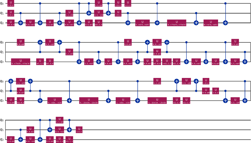
I understand that PauliDecompose exists and you can use a multiplexor to make multiple control, but after creating that QuantumCircuitOperator with ancillary, multiplexor (which was the giant circuit diagram), can you further decompose the circuit operators into a basis set of gates (ex: say your basis is X,Y,Z,CNOT,T)?
I understand that PauliDecompose exists and you can use a multiplexor to make multiple control, but after creating that QuantumCircuitOperator with ancillary, multiplexor (which was the giant circuit diagram), can you further decompose the circuit operators into a basis set of gates (ex: say your basis is X,Y,Z,CNOT,T)?
You can use Qiskit's transpilation for it, here is an example:
In[]:=
QuantumCircuitOperator["Multiplexer"["X","Y","Z"]]["Qiskit"]["Decompose"]["Transpile",{"cx","u"}]
Out[]=
QiskitCircuit