Lichtenberg figures (https://en.wikipedia.org/wiki/Lichtenberg_figure) can be generated by irradiating e.g. PMMA (i.e. Poly(methyl methacrylate), “acrylic glass”) with a high energy electron beam. This way electrons are implanted inside the material - which is an insulator. By a controlled discharge very aesthetic tree structures consisting of tracks from the electrical current can be generated. (This is just one method.)
It is fun trying to imitate this using Mathematica! The idea is simple:
It is fun trying to imitate this using Mathematica! The idea is simple:
◼
define a MeshRegion (this is all you need as input);
◼
convert it to a Graph (with preserved VertexCoordinates and EdgeWeight);
◼
use FindShortestPath to a specific “starting point”.
Generating Lichtenberg like figure from MeshRegion in 2D or 3D:
Generating Lichtenberg like figure from MeshRegion in 2D or 3D:
In[]:=
meshRegion2Lichtenberg[mr_MeshRegion]:=Module[{pts,conns,coord2index,index2coord,geomStart,startPt,startPtIndex,edgeWeights,ue,numPoints,graph,shortestPath,lines},pts=MeshPrimitives[mr,0];pts=Chop@@@pts;(*points*)numPoints=Length[pts];conns=Chop@@@MeshPrimitives[mr,1];(*connections*)coord2index=MapIndexed[#1First[#2]&,pts];index2coord=Rule[#2,#1]&@@@coord2index;(*geometricstartpoint:middle/bottom*)geomStart=Append[Mean/@Most[#],Min[Last[#]]]&@CoordinateBounds[pts];(*meshpointwhichisclosestto"geomStart"forstart:*)startPt=First@TakeSmallestBy[pts,EuclideanDistance[geomStart,#]&,1];startPtIndex=startPt/.coord2index;edgeWeights=N[EuclideanDistance@@@conns];ue=UndirectedEdge@@@(conns/.coord2index);graph=Graph[Range[numPoints],ue,VertexCoordinatespts,EdgeWeightedgeWeights];shortestPath=FindShortestPath[graph,startPtIndex];lines=(Partition[#,2,1]&/@(shortestPath/@Complement[Range[numPoints],{startPtIndex}]))/.index2coord;(*statistics:"how many times is the line segment `used`:"*)Tally[Flatten[lines,1]]]
As mentioned there is a simple mapping from a MeshRegion to the Lichtenberg graphics:
In[]:=
(*exampleregions:*)reg1=BooleanRegion[And,{Disk[{0,.5},1],Disk[{-.5,-.2},1],Disk[{.5,-.2},1]}];mr1=DelaunayMesh[RandomPoint[reg1,3000]];reg2=ParametricRegion[{{s,(1+t)s^2-t},-1≤s≤1&&0≤t≤1},{s,t}];mr2=DiscretizeRegion[reg2,MaxCellMeasure{"Length".05}];reg3=BooleanRegion[Xor,{DiskSegment[{0,0},2,{-.3,Pi+.3}],BooleanRegion[Or,{Disk[{-.5,.9},.35],Disk[{.4,.5},.3]}]}];mr3=DiscretizeRegion[reg3,MaxCellMeasure{"Length".1}];(*regiontakenfromDocumentation/ParametricRegion/Scope:*)constraint=-3/4+(5*x-20*x^3+16*x^5)^2-(5*x-20*x^3+16*x^5)*(1-8*y^2+8*y^4)+(1-8*y^2+8*y^4)^2≤0;mr4=DiscretizeRegion[ImplicitRegion[constraint,{x,y}],MaxCellMeasure{"Length".05}];regions={mr1,mr2,mr3,mr4};
In[]:=
lichtenbergs=ParallelMap[(wlSegs=meshRegion2Lichtenberg[#];Graphics[{{Black,Thickness[Sqrt[#2]/2500],Line[#1]}&@@@wlSegs}])&,regions];
In[]:=
GraphicsGrid[Transpose[{regions,lichtenbergs}],FrameAll,ImageSize600]
Out[]=

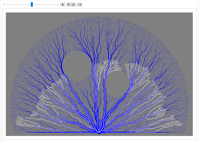
Single steps of function meshRegion2Lichtenberg for exporting animation:
Single steps of function meshRegion2Lichtenberg for exporting animation:
In[]:=
mr=DiscretizeRegion[reg3,MaxCellMeasure{"Length".07}];pts=MeshPrimitives[mr,0];pts=Chop@@@pts;numPoints=Length[pts];
In[]:=
conns=Chop@@@MeshPrimitives[mr,1];coord2index=MapIndexed[#1First[#2]&,pts];index2coord=Rule[#2,#1]&@@@coord2index;geomStart=Append[Mean/@Most[#],Min[Last[#]]]&@CoordinateBounds[pts];startPt=First@TakeSmallestBy[pts,EuclideanDistance[geomStart,#]&,1];startPtIndex=startPt/.coord2index;edgeWeights=N[EuclideanDistance@@@conns];ue=UndirectedEdge@@@(conns/.coord2index);
In[]:=
graph=Graph[Range[numPoints],ue,VertexCoordinatespts,EdgeWeightedgeWeights];shortestPath=FindShortestPath[graph,startPtIndex];
In[]:=
sp=(shortestPath/@Complement[Range[numPoints],{startPtIndex}]);
In[]:=
lines=(Partition[#,2,1]&/@sp)/.index2coord;wSegs=Tally[Flatten[lines,1]];
In[]:=
flash=Line/@(SortBy[sp,Length]/.index2coord);flash=Prepend[Partition[flash,150],{}];
In[]:=
Animate[Graphics[{{Blue,Thickness[Sqrt[#2]/2500],Line[#1]}&@@@wSegs,Thickness[.002],White,flash〚n〛},ImageSize700,BackgroundGray],{n,1,Length[flash],1},DisplayAllSteps->True,RefreshRate5]
Out[]=
Monitor[imgs=Table[Image@Graphics[{{Blue,Thickness[Sqrt[#2]/2500],Line[#1]}&@@@wSegs,Thickness[.002],White,flash〚n〛},ImageSize700,BackgroundGray],{n,1,Length[flash]}],N[n/Length[flash]]];
SetDirectory[NotebookDirectory[]];Export["lichtenberg.gif",imgs,"DisplayDurations".2,"AnimationRepetitions"->Infinity]
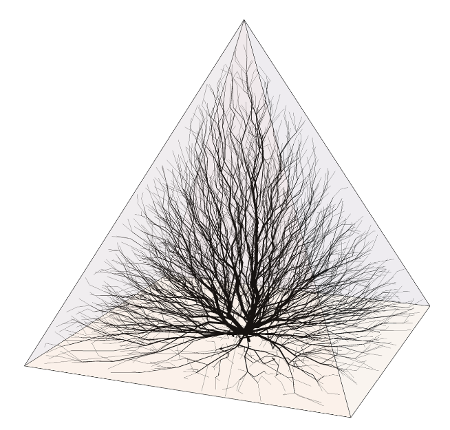
Example in 3D:
Example in 3D:
Due to the universally designed WL functions - it works in 3D without any change of code:
In[]:=
pts=RandomPoint[Pyramid[{{0,0,0},{2,0,0},{2,2,0},{0,2,0},{1,1,2}}],5000];mr=DelaunayMesh[pts];
In[]:=
wlSegs=meshRegion2Lichtenberg[mr];
In[]:=
Graphics3D[{Opacity[.1],Pyramid[{{0,0,0},{2,0,0},{2,2,0},{0,2,0},{1,1,2}}],{Opacity[1],Thickness[Sqrt[#2]/2500],Line[#1]}&@@@wlSegs},ImageSize700,BoxedFalse]
Out[]=
CITE THIS NOTEBOOK
CITE THIS NOTEBOOK
Computational Lichtenberg figures
by Henrik Schachner
Wolfram Community, STAFF PICKS, 2017
https://community.wolfram.com/groups/-/m/t/1065956
by Henrik Schachner
Wolfram Community, STAFF PICKS, 2017
https://community.wolfram.com/groups/-/m/t/1065956