Trie based classifiers evaluation
By Anton Antonov
MathematicaForPrediction at GitHub
MathematicaForPrediction at WordPress
July, August 2022

Introduction

In this notebook we show how to evaluate Machine Learning (ML) classifiers based on Tries with frequencies, [AA1, AA2, AAp1], created over a well known ML dataset. The computations are done with packages and functions from the Wolfram Language (WL) ecosystem.

The classifiers based on Tries with frequencies can be seen as generalized Naive Bayesian Classifiers (NBCs).

We use the workflow summarized in this flowchart:

In[]:=

Import["https://raw.githubusercontent.com/antononcube/MathematicaForPrediction/master/MarkdownDocuments/Diagrams/A-monad-for-classification-workflows/Classification-workflow-horizontal-layout.jpg"]

Out[]=

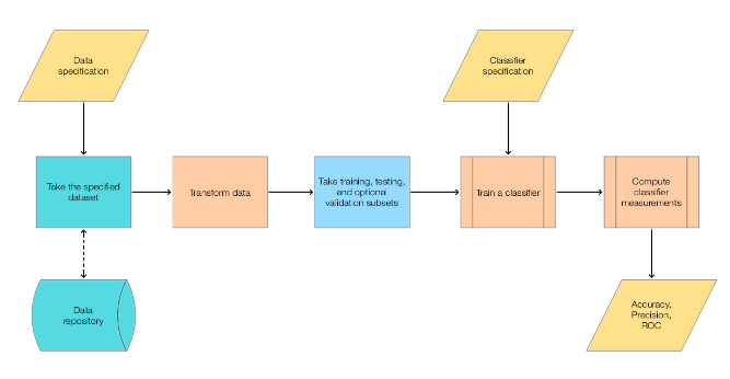
For more details on classification workflows see the article “A monad for classification workflows”, [AA3].

Remark: This notebook is the Mathematica counterpart of the Raku computable Markdown document with the same name [AA7, AA6].

Remark: Mathematica and WL are used as synonyms in this notebook.

Data

In this section we obtain a dataset to make classification experiments with.

Through the Wolfram Function Repository (WFR) function ExampleDataset we can get data for the Titanic ship wreck:

In[]:=

dsTitanic0=ResourceFunction["ExampleDataset"][{"MachineLearning","Titanic"}];dsTitanic0〚1;;4〛

Out[]=

passenger class	passenger age	passenger sex	passenger survival
1st	29.0	female	survived
1st	0.9167	male	survived
1st	2.0	female	died
1st	30.0	male	died

Remark: ExampleDataset uses ExampleData. Datasets from the ExampleData's "MachineLearning" and "Statistics" collections are processed in order to obtain Dataset objects.

Instead of using the built-in Titanic data we use a version of it (which is used in Mathematica-vs-R comparisons, [AAr1]):

In[]:=

dsTitanic〚1;;4〛

Out[]=

id	passengerClass	passengerAge	passengerSex	passengerSurvival
1	1st	30	female	survived
2	1st	0	male	survived
3	1st	0	female	died
4	1st	30	male	died

Here is a summary of the data:

In[]:=

ResourceFunction["RecordsSummary"][dsTitanic]

Out[]=



1 id

Min	1
1st Qu	327.75
Mean	655
Median	655
3rd Qu	982.25
Max	1309

2 passengerClass

3rd	709
1st	323
2nd	277

3 passengerAge

Min	-1
1st Qu	10
Median	20
Mean	23.55
3rd Qu	40
Max	80

4 passengerSex

male	843
female	466

5 passengerSurvival

died	809
survived	500



Make tries

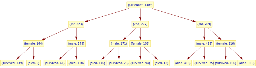
In this section for demonstration purposes let us create a shorter trie and display it in tree form.

Here we drop the identifier column and take the record fields in a particular order, in which "passengerSurvival" is the last field:

In[]:=

lsRecords=Normal@dsTitanic[All,Prepend[KeyDrop[#,"id"],"passengerAge"->ToString[#passengerAge]]&][All,{"passengerClass","passengerSex","passengerAge","passengerSurvival"}][Values];

Here is a sample:

In[]:=

RandomSample[lsRecords,3]

Out[]=

{{3rd,male,20,died},{3rd,male,70,died},{3rd,male,-1,died}}

Here make a trie without the field "passengerAge":

In[]:=

trTitanic=TrieCreate[lsRecords〚All,{1,2,4}〛];TrieForm[trTitanic,AspectRatio->1/4,ImageSize->900]

Out[]=

Here is a corresponding mosaic plot, [AA4, AAp3]:

In[]:=

MosaicPlot[lsRecords〚All,{1,2,4}〛]

Out[]=

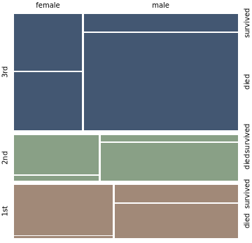
Remark: The function MosaicPlot uses tries with frequencies in its implementation. Observing and reasoning with mosaic plots should make it clear that tries with frequencies are (some sort of) generalized Naive Bayesian classifiers.

Trie classifier

In this section we create a Trie-based classifier.

In order to make certain reproducibility statements for the kind of experiments shown here, we use random seeding (with SeedRandom) before any computations that use pseudo-random numbers. Meaning, one would expect WL code that starts with a SeedRandom statement (e.g. SeedRandom[89]) to produce the same pseudo random numbers if it is executed multiple times (without changing it.)

In[]:=

SeedRandom[12];

Here we split the data into training and testing data in a stratified manner (a split for each label):

In[]:=

aSplit1=GroupBy[lsRecords,#〚-1〛&,AssociationThread[{"training","testing"},TakeDrop[RandomSample[#],Round[0.75*Length[#]]]]&];Map[Length,aSplit1,{2}]

Out[]=

survivedtraining375,testing125,diedtraining607,testing202

Here we aggregate training and testing data (and show the corresponding sizes):

In[]:=

aSplit2=<|"training"->Join@@Map[#training&,aSplit1],"testing"->Join@@Map[#testing&,aSplit1]|>;Length/@aSplit2

Out[]=

training982,testing327

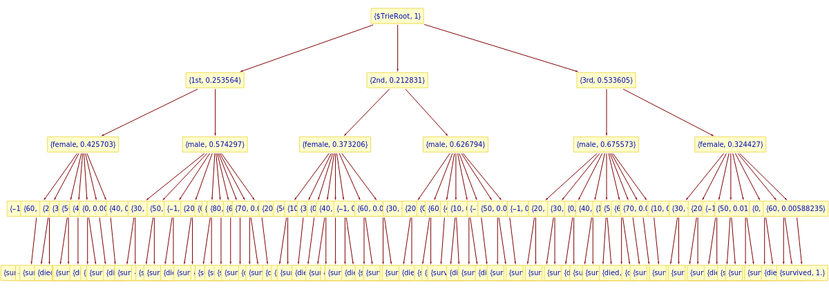
Here we make a trie with the training data (and show the node counts):

In[]:=

trTitanic=TrieNodeProbabilities[TrieCreate[aSplit2["training"]]];TrieNodeCounts[trTitanic]

Out[]=

total142,internal60,leaves82

Here is the trie in tree form:

In[]:=

TrieForm[trTitanic,ImageSize->1200,AspectRatio->1/3]

Out[]=

Here is an example decision-classification:

In[]:=

TrieClassify[trTitanic,{"1st","female"}]

Out[]=

survived

Here is an example probabilities-classification:

In[]:=

TrieClassify[trTitanic,{"1st","female"},"Probabilities"]

Out[]=

survived0.962264,died0.0377358

We want to classify across all testing data, but not all testing data records might be present in the trie. Let us check that such testing records are few (or none):

In[]:=

Tally[Map[TrieKeyExistsQ[trTitanic,#]&,aSplit2["testing"]]]

Out[]=

{{True,321},{False,6}}

Let us remove the records that cannot be classified:

In[]:=

lsTesting=Pick[aSplit2["testing"],Map[TrieKeyExistsQ[trTitanic,#]&,aSplit2["testing"]]];Length[lsTesting]

Out[]=

321

Here we classify all testing records and show a sample of the obtained actual-predicted pairs:

In[]:=

lsClassRes={Last[#],TrieClassify[trTitanic,Most[#]]}&/@lsTesting;RandomSample[lsClassRes,6]

Out[]=

{{survived,survived},{died,survived},{died,died},{survived,survived},{survived,died},{survived,survived}}

Here we cross tabulate the actual vs predicted labels using WFR's CrossTabulate:

In[]:=

ResourceFunction["CrossTabulate"][lsClassRes]

Out[]=

	died	survived
died	186	12
survived	52	71

The cross-tabulation results look bad because the default decision threshold is used. We get better results by selecting a decision threshold via Receiver Operating Characteristic (ROC) plots.

Trie classification with ROC plots

In this section we systematically evaluate the Trie-based classifier using the Receiver Operating Characteristic (ROC) framework.

Here we classify all testing data records. For each record:

◼

Get probabilities association

◼

Add to that association the actual label

◼

Make sure the association has both survival labels

In[]:=

lsClassRes=Map[Join[<|"survived"->0,"died"->0,"actual"->#〚-1〛|>,TrieClassify[trTitanic,#〚1;;-2〛,"Probabilities"]]&,lsTesting];

Here we make a ROC record, [AA5, AAp4]:

In[]:=

ToROCAssociation[{"survived","died"},#actual&/@lsClassRes,Map[If[#survived≥0.5,"survived","died"]&,lsClassRes]]

Out[]=

TruePositive71,FalsePositive14,TrueNegative184,FalseNegative52

Here we obtain the range of the label “survived”:

In[]:=

lsVals=Map[#survived&,lsClassRes];MinMax[lsVals]

Out[]=

{0,1.}

Here we make list of decision thresholds:

In[]:=

lsThresholds=N@RangeMin[lsVals],Max[lsVals],

;

In the following code cell for each threshold:

◼

For each classification association decide on “survived” if the corresponding value is greater or equal to the threshold

◼

Make threshold’s ROC-association

In[]:=

lsROCs=Table[ToROCAssociation[{"survived","died"},#actual&/@lsClassRes,Map[If[#survived≥th,"survived","died"]&,lsClassRes]],{th,lsThresholds}];

Here is the obtained ROCs dataset:

In[]:=

Dataset[MapThread[Prepend[#1,"Threshold"->#2]&,{lsROCs,lsThresholds}]]

Out[]=

Threshold	TruePositive	FalsePositive	TrueNegative	FalseNegative
0.0	123	198	0	0
0.0333333	123	188	10	0
0.0666667	123	182	16	0
0.1	123	182	16	0
0.133333	116	112	86	7
0.166667	116	112	86	7
0.2	105	56	142	18
0.233333	101	47	151	22
0.266667	101	47	151	22
0.3	96	42	156	27
0.333333	86	31	167	37
0.366667	86	31	167	37
0.4	82	27	171	41
0.433333	82	22	176	41
0.466667	80	17	181	43
0.5	71	14	184	52
0.533333	71	12	186	52
0.566667	71	12	186	52
0.6	61	3	195	62
0.633333	61	3	195	62
rows 1–20 of 31

Here is the corresponding ROC plot:

In[]:=

ROCPlot["FPR","TPR",lsThresholds,lsROCs,GridLines->Automatic,ImageSize->Large]

Out[]=

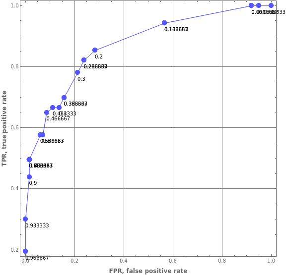
We can see the Trie-based classifier has reasonable prediction abilities -- we get ≈ 80% True Positive Rate (TPR) for a relatively small False Positive Rate (FPR), ≈ 20%.

Confusion matrices

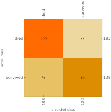
Using ClassifierMeasurements we can produce the corresponding confusion matrix plots (using "made on the spot" Manipulate interface):

In[]:=

DynamicModule[{lsThresholds=lsThresholds,lsClassRes=lsClassRes,lsClassRes2},Manipulate[lsClassRes2=Map[{#actual,If[#survived≥lsThresholds〚i〛,"survived","died"]}&,lsClassRes];Append[DeleteCases[ClassifierMeasurements[lsClassRes2〚All,1〛,lsClassRes2〚All,2〛,"ConfusionMatrixPlot"],ImageSize->_],ImageSize->Medium],{{i,Flatten[Position[lsThresholds,Nearest[lsThresholds,0.3]〚1〛]]〚1〛,"index:"},1,Length[lsThresholds],1,Appearance->"Open"},{{normalizeQ,False,"normalize?:"},{False,True}}]]

Out[]=

index:

normalize?:

References

Setup

In[]:=

Import["https://raw.githubusercontent.com/antononcube/MathematicaForPrediction/master/TriesWithFrequencies.m"];Import["https://raw.githubusercontent.com/antononcube/MathematicaForPrediction/master/ROCFunctions.m"];Import["https://raw.githubusercontent.com/antononcube/MathematicaForPrediction/master/MosaicPlot.m"];

In[]:=

dsTitanic=Import["https://raw.githubusercontent.com/antononcube/MathematicaVsR/master/Data/MathematicaVsR-Data-Titanic.csv","Dataset",HeaderLines->1];

Introduction

Data

Make tries

Trie classifier

Trie classification with ROC plots

Confusion matrices

References

Articles

Packages

Repositories

Setup