CITE THIS NOTEBOOK: What Is the Shape of a Cupola? by Rafael López. Wolfram Community MAR 14 2022.
ORIGINAL ARTICLE: Rafael López (2023) What Is the Shape of a Cupola?, The American Mathematical Monthly, 130:3, 222-238, https://doi.org/10.1080/00029890.2022.2154557.
ORIGINAL ARTICLE: Rafael López (2023) What Is the Shape of a Cupola?, The American Mathematical Monthly, 130:3, 222-238, https://doi.org/10.1080/00029890.2022.2154557.
Article Abstract: This article examines the shape of a surface obtained by a hanging flexible, inelastic material with prescribed area and boundary curve. The shape of this surface, after being turned upside down, is a model for cupolas (or domes) under the simple hypothesis of compression. Investigating the rotational examples, we provide and illustrate a novel design for a roof that has the extraordinary property that its shape, although natural, is modeled by a surface of revolution whose axis of rotation is horizontal.
Introduction
Introduction
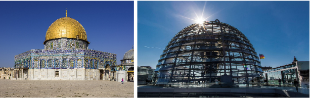
The aim of this project is to discuss three mathematical approaches of the shape of a dome, beginning with the ideal model and comparing with two known surfaces, the catenary rotation surface and the paraboloid. The surface that models a rotational dome is called a rotational tectum. In Figure 1 we see two domes which can be viewed as surfaces of revolution with respect to a vertical axis. Under ideal conditions, the rotational tectum is the surface with the lowest center of gravity among all surfaces with the same area and the same boundary curve. In this work, we compare numerically how far are the energies between the ideal model and the other two surfaces [4].Figure 1. Left: the Dome of the Rock, Jerusalem. Right: the Bundestag, Berlin ([1]).
The Rotational Tectum and the Two Non-Ideal Models
The Rotational Tectum and the Two Non-Ideal Models
It is well known that the shape of a hanging flexible chain suspended from its endpoints is the catenary. The two-dimensional analogue is a bounded piece S of homogeneous flexible material of given area hanging from its boundary curve and suspended by its weight. In a position of static equilibrium, the tension forces exerted on the surface S only have tangential components [2,3]. Therefore, if we turn S upside down, these forces become only internal compressive forces. In consequence these surfaces are models of domes and roofs and with a consequent reduction of collapse. Under ideal conditions in the construction of domes, the energy is the weight of the surface and it is expressed by the height of the center of gravity of the dome. The Lagrange conditions are the area of the dome together its boundary curve . If S is given as the graph z=u(x,y), then this energy isJ[S]=σu,where the first summand is the height of the center of gravity, σ is the area density, |Du|= + and the second summand is the Lagrange constraint given by the area of S. Assuming σ=1 and after a vertical translation, the Euler-Lagrange equation is div=We now consider a dome or cupola of rotational shape. Assume that the z-axis is the rotational axis and that the dome is parametrized by X(r,θ)=(r cosθ,r sinθ,u(r)). Consider a bounded piece S of a dome bounded by a horizontal circle of radius R >0 and height z=u(R). This surface, a rotational tectum, is determined by the generating curve r ↦ (r,0,u(r)) contained in the xz-plane and the Euler-Lagrange writes now as (1) += where r∈ [0,R]. This equation cannot solved explicitly by quadratures and we need to use numerical methods to get solutions. On the other hand, there another two surfaces of revolution which, not solving (1), may be candidates to the model of a rotational dome. The first surface is the catenary rotation surface. This surface is obtained by rotating a vertical catenary with respect to its rotation axis. The reason to study this surface is because the catenary is the model of an arch, so rotating about its symmetry axis, we obtain a surface of revolution that could be model of a dome. The second candidate is the paraboloid, the rotational surface obtained by rotating a vertical parabola z(x)=c +m with respect to its symmetric axis. The motivation has its origin in the well-known dispute between parabolas and catenaries in the construction of arches. Furthermore, the paraboloid has a clear advantage from the architectural viewpoint because this surface is defined with polynomials, in contrast to the catenary that uses exponential functions.
A
0
Γ
A
0
Γ
∫
S
1+|Du
+λ2
|
∫
S
1+|Du
2
|
2
2
(u)
∂
x
2
(u)
∂
y
Du
1+|Du
2
|
1
u
1+|Du
2
|
Γ
R
′′
u
1+
′2
u
′
u
r
1
u
z(x)=+m
Cosh(cx)
c
2
x
Implementation with Mathematica
Implementation with Mathematica
Consider u=u(r) a solution of (1) with initial conditions (2) u(0)=u0, u’(0)=0, defined in the interval [0,R]. Let T denote the rotational tectum obtained by rotating z=u(r) about the z-axis. The boundary curve of T is the horizontal circle (3) = {(x,y,u(R)): +=}, where u(R)>0 is the height of . The area of T is(4) = and the height of its center of gravity is (5) = xu(x) Let now the catenary rotation surface with the same area and boundary curve. The generating catenary is(6) [x]=+m, x∈ [0,R], where c and m and real numbers and c>0. Let denote the corresponding rotational catenary obtained when we rotate with respect to the z-axis. We will choose the values c and m in (6) so the area of is and its boundary is . The last condition implies (7) . The area of is obtained by quadratures, (8) = Finally, the height of the center of gravity of is (9) = = + m It is important to point out that the derivation of (8) and (9) are obtained directly from Mathematica with the function Integrate. To derive the parameters c and m from (7) and (8), it is enough with the command FindRoot. In the case of paraboloids, the methodology is analogous. Consider the parabola (x) = c x^2 + m, x∈ [0,R], where c and m are real numbers, c>0, and situated in the coordinate xz-plane. Let be the paraboloid obtained by rotating about the z-axis. Let be the height of the center of gravity. Since the boundary is , we have the condition(10) c R^2 + m = u(R). The area of is(11) = and the height of its center of gravity is(12) == + m As it is expectable, all expressions for the paraboloid are polynomial in the variables c and R which, from the computational and architectural viewpoint, is much manageable. Again, the function Integrate allows to solve both integrals. We show the values of in Table 1. We use Mathematica to compute the area (4) and the center of gravity (5) of the rotational tectum. The steps to follow are:
Γ
R
2
x
2
y
2
R
Γ
R
A
0
A
0
2πx
R
∫
0
1+
x′
u
2
(x)
h
T
h
T
2π
A
0
R
∫
0
1+
x′
u
2
(x)
z
c,m
Cosh[cx]
c
C
c,m
z
c,m
C
c,m
A
0
Γ
R
m+=u[R]
Cosh[cR]
c
C
c,m
A
0
2πx
R
∫
0
1+
x=′
z
c,m
2
(x)
2π(cRsinh[cR]-cosh[cR]+1)
2
c
h
C
C
c,m
h
c
2πx(x)
R
∫
0
z
c,m
1+(x)^2
x′
z
c,m
A
0
π(2+2cRsinh[2cR]-cosh[2cR]+1)
2
c
2
R
4
3
c
A
0
p
c,m
P
c,m
p
c,m
h
P
Γ
R
P
c,m
A
0
2πx
R
∫
0
1+
x=′
p
c,m
2
(x)
π-1
3/2
(4+1)
2
c
2
R
6
2
c
h
P
h
P
2πx(x)
R
∫
0
p
c,m
1+(x)^2
x′
p
c,m
A
0
π(6-1)+1
2
c
2
R
3/2
(4+1)
2
c
2
R
60
3
c
A
0
h
P
1
.Fix >0 in (2), the lowest point of T, and by numerical methods, we solve (1)-(2).
u
0
2
.Fix R>0 and let [0,R] be the domain of u which determines the rotational tectum T. With this value for R, we prescribe , the boundary curve of T, which it is a data in the problem.
Γ
R
3
.Compute the area using (4).
A
0
4
.Calculate the parameters c and m of in order that its area is and its boundary is . Here we use (7) and (8).
C
c,m
A
0
Γ
R
5
.Using (5) and (9), compute the values of the heights and of the centers of gravity of T and , respectively.
h
T
h
C
C
c,m
6
.For the paraboloids, we calculate the parameters c and m by using (10) and (11) and the value by means of (12).
h
P
Table 1: Comparison of , and when the lowest height of T is = 1.
h
T
h
C
h
P
u
0
R | u(R) | A 0 | h T | h C | % hc-ht u[R]- u 0 | h P | % hc-hp u[R]- u 0 |
2 | 1.8854 | 14.63 | 1.4773 | 1.4782 | 0.0969 | 1.4778 | 0.0482 |
4 | 3.7295 | 66.22 | 2.5786 | 2.58811 | 0.3488 | 2.5843 | 0.2119 |
6 | 5.7681 | 155.99 | 3.8651 | 3.8887 | 0.4942 | 3.8805 | 0.3232 |
8 | 7.8292 | 155.99 | 5.1997 | 5.2377 | 0.5573 | 5.2253 | 0.3753 |
10 | 9.8837 | 444.43 | 6.5477 | 6.5994 | 0.5819 | 6.5830 | 0.3975 |
12 | 11.9278 | 642.08 | 7.8989 | 7.9632 | 0.5891 | 7.9430 | 0.4046 |
14 | 13.9628 | 875.13 | 9.2498 | 9.3261 | 0.5887 | 9.3023 | 0.4057 |
16 | 15.9903 | 1143.55 | 10.5993 | 10.6870 | 0.5849 | 10.6598 | 0.4033 |
18 | 18.0120 | 1447.30 | 11.9471 | 12.0458 | 0.5798 | 12.0152 | 0.4002 |
20 | 20.0290 | 1786.39 | 13.2932 | 13.4025 | 0.5744 | 13.3686 | 0.3962 |
Without loss of generality, we fix =1 as initial condition (2). In Table 1, we show the comparison of the value and for values R between R=2 and R=20. In order to relate and , we show the percentage between the difference - with the height u(R)-u(0) of the rotational tectum.
We write down the Mathematica codes employed to obtain Table 1. First we solve the equation (7) of the rotational tectum. Since the equation (1) of the rotational tectum has a singular point at x = 0, we modify the initial condition to be close to 0 by putting = 0.000001. The initial conditions are u () = , with = 1, and u’() = 0. The value of the radius of the boundary circle is R. In the next code lines, the input R is R = 2.
u
0
h
T
h
C
h
T
h
C
h
C
h
T
We write down the Mathematica codes employed to obtain Table 1. First we solve the equation (7) of the rotational tectum. Since the equation (1) of the rotational tectum has a singular point at x = 0, we modify the initial condition to be close to 0 by putting
r
0
r
o
u
0
u
0
r
0
(* Solving the rotational tectum *)ro=0.000001;R=2;uo=1;sol=NDSolve[{u''[x]/(1+u'[x]^2)+u'[x]/x1/u[x],u[ro]uo,u'[ro]0},u[x],{x,ro,R}];uu[x_]=u[x]/.sol[[1]];
We compute the area of the rotational tectum with the formula (4):
A
0
(* area of the rotational tectum *)Ao=NIntegrate[2Pi x Sqrt[1+uu'[x]^2],{x,ro,R}]
14.634
Next, compute the height of the center of gravity of the rotational tectum using (5):
(* height of the center of gravity of the rotational tectum *)hs=NIntegrate[2Pi uu[x]x Sqrt[1+uu'[x]^2],{x,ro,R}]/Ao
1.47735
With the value , we calculate the parameters c and m of the catenary using \eqref (7) and (8). First, we introduce the equation of the catenary :
A
0
C
c,m
(* The equation of the catenary *)z[x_]:=1/c Cosh[c x]+m
In Mathematica, we use the function FindRoot to find c and m:
(* Finding the parameters c and m for the rotational catenary *)variables=FindRoot[{z[R]uu[R],2Pi (c R Sinh[c R]-Cosh[c R]+1)/c^2Ao},{{c,.3},{m,-4}}];
We compute the height of the center of gravity of the catenary rotation surface according to (9).
h
C
(* height of the center of gravity of the rotational catenary *)hc=Pi (2 c^2 R^2+2 c R Sinh[2 c R]-Cosh[2 c R]+1)/(4 c^3 Ao)+m/.variables
1.47821
We calculate the deviation of the value with in relation with the height of the rotational tectum. We use the function Nintegrate.
h
C
h
T
(* deviation with respect to the height of the surface *)(hc-hs)/(uu[R]-1) 100
0.0969406
The Mathematica codes for the paraboloids are similar.
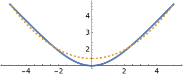
In Figures 2 and 3 we show some pictures of rotational tectums, catenary rotational surfaces and paraboloids with the same boundary and area.
In Figures 2 and 3 we show some pictures of rotational tectums, catenary rotational surfaces and paraboloids with the same boundary and area.
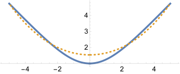
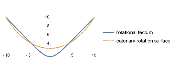
Figure 2. Comparison between rotational tectums (thick) and catenary rotation surfaces (dashed). Left: R = 5 where = 3.2115 and = 3.2278. Right: R = 10, = 6.5477 and = 6.5994.
h
T
h
C
h
T
h
C
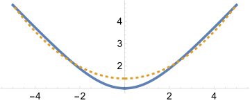
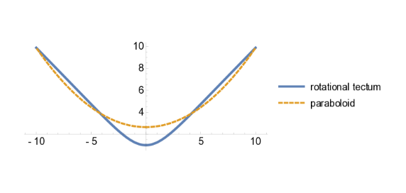
Figure 3. Comparison between rotational tectums (thick) and paraboloids (dashed). Left: R = 5 where = 3.2115 and = 3.2219. Right: R = 10, = 6.5477 and = 6.5994.
h
T
h
P
h
T
h
P
(* The equation of the catenary *)z[x_]:=1/a Cosh[a x]+m(* The equation of the parabola *)p[x_]:=a x^2+m(* Solving the rotational tectum equation. Here R=5 *) xo=0.000001;ro=5;zo=1;sol=NDSolve[ {u''[x]/(1+u'[x]^2)+u'[x]/x1/ u[x] ,u[xo]zo,u'[xo]0}, u[x],{x,xo,ro}];uu[x_]=u[x]/.sol[[1]]; (* height of the surface *)uu[ro] (* area of the surface *)Ao=NIntegrate[2Pi x Sqrt[1+uu'[x]^2],{x,xo,ro}] (* Finding the parameters a and m for the rotational catenary *)variables1=FindRoot[{z[ro]uu[ro],2Pi(a ro Sinh[a ro]-Cosh[a ro]+1)/a^2Ao},{{a,.3},{m,-4}}];(* Finding the parameters a and m for the paraboloid *)variables2=FindRootp[ro]uu[ro],Ao,{{a,.3},{m,-4}};(* height of the center of gravity of the rotational catenary *)cgrotcatenary=Pi(2 a^2 ro^2+2 a ro Sinh[2 a ro]-Cosh[2 a ro]+1)/(4 a^3 Ao)+m/.variables1(* height of the center of gravity of the paraboloid *)+m/.variables2
π -1+
3/2
(1+4 )
2
a
2
ro
6
2
a
π 1+ (-1+6 )
3/2
(1+4 )
2
a
2
ro
2
a
2
ro
60 Ao
3
a
4.74158
106.464
3.22784
3.2219
Plotting the rotational tectum and the paraboloid: Figure 3
f1=ParametricPlot[{Evaluate[{-x,u[x]}/.sol],Evaluate[{-x,p[x]}/.variables2]},{x,xo,ro},PlotRange->All,PlotStyle{{Thickness[0.01]},{Thickness[.008], Dashed}},LabelStyle{FontFamily"Arial",FontSize14,Black},PlotLegends{"rotational tectum","paraboloid"}];f2=ParametricPlot[{Evaluate[{x,u[x]}/.sol],Evaluate[{x,p[x]}/.variables2]},{x,xo,ro},PlotRange->All,PlotStyle{{Thickness[0.01]},{Thickness[.008], Dashed}},LabelStyle{FontFamily"Arial",FontSize14,Black}];Show[f2,f1]
Results
Results
1
.As it is expectable, the heights and are higher than . However the differences - and - are very small. In terms of percentages in relation with the total height of the rotational tectum T, the deviation is less than 0 .60% for all values of R in the first case and less than 0 .41% in the case of paraboloids.
h
C
h
P
h
T
h
C
h
T
h
P
h
T
2
.Both deviation percentages attain a maximum at R=12 and next decreases.
3
.The approximation of the paraboloid to the rotational tectum is better than the catenary rotation surface because < for all values of R. This is surprising and contrasts with the reverse property between the centers of gravity of the catenary and the parabola.
h
P
h
C
4
. A parallel discussion comparing the three surfaces is the relation between the lowest points of the surface. In the rotational dome this point corresponds with . An analysis of the lowest points and of the catenary rotation surfaces and paraboloids, respectively, shows that < and < . This is expectable although there is not an a priori relation between the centers of gravity and the lowest points. Moreover, one proves that < , showing again that paraboloids adjust better to the rotational tectums than the catenary rotation surfaces. See Table 2.
u
0
w
C
w
P
u
0
w
C
u
0
w
P
w
P
w
C
5
.The deviations - and - increase as R ∞ and are significant. This contrasts with the differences - and -.Thus the top of the (inverted) catenary rotation surface or the paraboloid are clearly below that of the rotational tectum.
w
C
w
T
w
P
w
T
h
C
h
T
h
P
h
T
Table 2: Comparison of , and the lowest height =1 of the rotational tectum T.
W
C
W
P
u
0
R | u(R) | A 0 | W C | % wc- u 0 u[R]- u 0 | W P | % wp- u 0 u[R]- u 0 |
2 | 1.8854 | 14.63 | 1.0452 | 5.1079 | 1.0318 | 3.5900 |
4 | 3.7295 | 66.22 | 1.3236 | 11.8550 | 1.2565 | 9.3987 |
6 | 5.7681 | 155.99 | 1.7781 | 16.3190 | 1.6501 | 13.6348 |
8 | 7.8292 | 282.30 | 2.3128 | 19.2236 | 2.1270 | 16.5027 |
10 | 9.8837 | 444.43 | 2.8847 | 21.2156 | 2.6442 | 18.5085 |
12 | 11.9278 | 642.08 | 3.4751 | 22.6495 | 3.1822 | 19.9690 |
14 | 13.9628 | 875.13 | 4.0751 | 23.7228 | 3.7313 | 21.0701 |
16 | 15.9903 | 1143.55 | 4.6803 | 24.5515 | 4.2866 | 21.9246 |
18 | 18.0120 | 1447.30 | 5.2883 | 25.2075 | 4.8453 | 22.6035 |
20 | 20.0290 | 1786.39 | 5.8976 | 25.7377 | 5.4059 | 23.1536 |
Conclusions
Conclusions
As far the author knows, catenary rotation surfaces and paraboloids have not been tested in relation with the centers of gravity nor in comparison with the ideal model of the rotational tectum. It is known that the paraboloid is as an example of a quadric employed in architecture but without to clearly state what is its utility other than they are more tractable in the computational treatment of the design in construction (which is not a minor matter). From our conclusions, we give the following consequence in plain language and easy to understand:
Catenary rotation surfaces and paraboloids are surfaces that ‘adjust extremely well' to the ideal model of a rotational dome, being the paraboloid better than the catenary rotation surface.
Catenary rotation surfaces and paraboloids are surfaces that ‘adjust extremely well' to the ideal model of a rotational dome, being the paraboloid better than the catenary rotation surface.
References
References
[1] The photo of the Dome of the Rock is obtained from Wikipedia (commons.wikimedia.org/wiki/File : Jerusalem - 2013 (2) - Temple Mount - Dome of the Rock (SE exposure).jpg). The second image is obtained from https : // www.bundestag.de/en/visittheBundestag/dome/registration - 245686, copyright by Deutscher Bundestag/Neuhauser.
[2] Böhme, R., Hildebrandt, S., Taush, E.: The two-dimensional analogue of the catenary. Pacific J. Math. 88, 247- 278 (1980)
[3] López, R.: What is the Shape of a Cupola? Amer.Math.Monthly, to appear.
[4] López, R.: Comparison analysis between catenary rotation surfaces, paraboloids and surfaces subjected to compression forces, preprint (2022)