Abstract: The Wolfram Models are a discrete spacetime formalism represented by hypergraphs and causal graphs generated by simple computational rules. Given that these models represent spacetime, they can readily be used as spatial and temporal discretizations for numerically computing Partial Differential Equations (PDEs), which can prove useful in cases where the discretizations are too computationally expensive or difficult to produce.
This project is a preliminary study on ways the hypergraphs with interesting limiting geometries can be converted into a mesh for solving PDEs.
This project is a preliminary study on ways the hypergraphs with interesting limiting geometries can be converted into a mesh for solving PDEs.
When considering mathematical tools that are used in modelling, PDEs are arguably the most ubiquitous. However, they are incredibly difficult, if not impossible, to solve analytically, which forces us to turn to numerical algorithms to compute them.
Although there are various numerical methods used to solve PDEs, they usually come with their own set of challenges and limitations. When considering mesh-based methods specifically (i.e. finite difference or finite element methods), the construction of a mesh, particularly for domains with a complex geometry, is a computationally heavy task. Here, we look into the hypergraphs generated by the Wolfram models as possible discretizations or meshes that can be used directly by such methods. The primary advantage of this is, if the Wolfram Model effectively models spacetime, then these discretizations would save a large amount of computational effort in generating meshes used for PDEs that model physical phenomena.This is due to the fact that the Wolfram models are already discrete models, so they can be used as a “ready-made” tool to handle this.
This work aims to present a short demonstration of using the hypergraphs as a mesh for solving PDEs. Firstly, we start with the Poisson equation, a relatively easy equation to solve, and a given hypergraph generated from the Wolfram models. The hypergraph would then be converted into a graph and embedded into the Cartesian plane (to coordinatize it), and then be used to generate a mesh. The equation would then be solved using tools provided by Mathematica (i.e.NDSolve) on the given mesh. Secondly, we present a solution of the 2D Burgers' equation to demonstrate further the ability of these meshes to capture characteristics of some PDEs, such as the formation of shock waves.
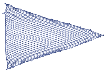
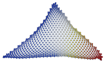
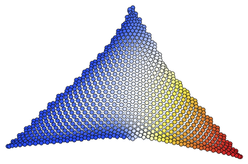
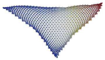
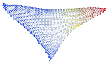
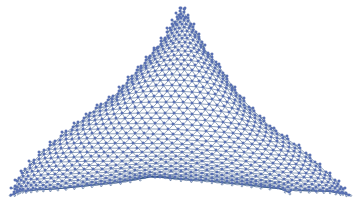
The work starts by presenting one example of a hypergraph that can act as the spatial discretization for the system. Consider the following hypergraph:
Although there are various numerical methods used to solve PDEs, they usually come with their own set of challenges and limitations. When considering mesh-based methods specifically (i.e. finite difference or finite element methods), the construction of a mesh, particularly for domains with a complex geometry, is a computationally heavy task. Here, we look into the hypergraphs generated by the Wolfram models as possible discretizations or meshes that can be used directly by such methods. The primary advantage of this is, if the Wolfram Model effectively models spacetime, then these discretizations would save a large amount of computational effort in generating meshes used for PDEs that model physical phenomena.This is due to the fact that the Wolfram models are already discrete models, so they can be used as a “ready-made” tool to handle this.
This work aims to present a short demonstration of using the hypergraphs as a mesh for solving PDEs. Firstly, we start with the Poisson equation, a relatively easy equation to solve, and a given hypergraph generated from the Wolfram models. The hypergraph would then be converted into a graph and embedded into the Cartesian plane (to coordinatize it), and then be used to generate a mesh. The equation would then be solved using tools provided by Mathematica (i.e.NDSolve) on the given mesh. Secondly, we present a solution of the 2D Burgers' equation to demonstrate further the ability of these meshes to capture characteristics of some PDEs, such as the formation of shock waves.
The work starts by presenting one example of a hypergraph that can act as the spatial discretization for the system. Consider the following hypergraph:
g1=ResourceFunction["WolframModel"][{{x,y,y},{z,x,u}}{{y,v,y},{y,z,v},{u,v,v}},{{0,0,0},{0,0,0}},1000,"FinalState"]G1=ResourceFunction["WolframModelPlot"][g1]
Out[]=
Out[]=
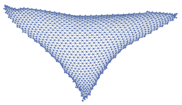
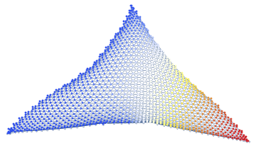
In order for us to use this hypergraph, we need to convert it into a graph first before creating a mesh out of it. After it's converted into a graph, it's embedded onto the Cartesian plane and then scaled down to fit what would be a sensible domain for the Poisson equation. This would look like:
Gr=ResourceFunction["HypergraphToGraph"][g1]C1=GraphEmbedding[Gr]C1=C1/(Mean[C1[[All,1]]])C1=#-{Mean[C1[[All,1]]],Mean[C1[[All,2]]]}&/@(C1)ListPlot[C1]
Out[]=
Out[]=
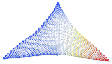
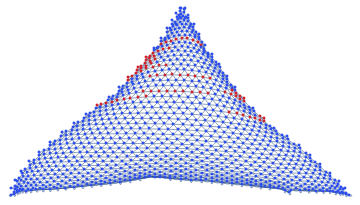
Now, the graph is ready to be converted into a mesh:
Mesh1=ResourceFunction["NonConvexHullMesh"][C1,0.2]
Out[]=
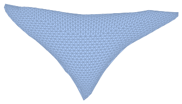
And now we have a mesh ready to be used!
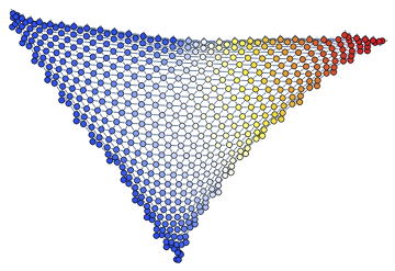
The next step is to define the Poisson equation in Mathematica and use NDSolve to solve it.
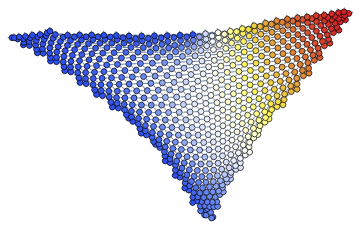
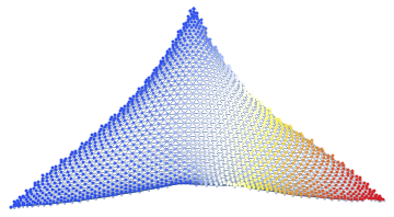
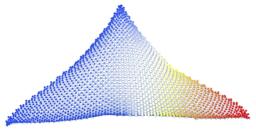
Furthermore, with the solutions obtained from NDSolve, we assign those values to the vertices of the graph and code it with a temperature map. The final graph is colored according to a temperature map, so the warmer the color, the higher the value of the PDE is at that point.
The next step is to define the Poisson equation in Mathematica and use NDSolve to solve it.
Furthermore, with the solutions obtained from NDSolve, we assign those values to the vertices of the graph and code it with a temperature map. The final graph is colored according to a temperature map, so the warmer the color, the higher the value of the PDE is at that point.
ClearAll[x];ClearAll[y]op=-Laplacian[u[x,y],{x,y}]-5Bndry=DirichletCondition[u[x,y]==1,x≤0]ufun=NDSolveValue[{op==0,Bndry},u[x,y],{x,y}∈Mesh1]VertexWeightValues={}For[i=1,i<VertexCount[Gr]+1,i++,x=C1[[i]][[1]];y=C1[[i]][[2]];VertexWeightValues={VertexWeightValues,ufun}]VertexWeightValues=VertexWeightValues//FlattenWGraph1=Graph[Gr,VertexWeightVertexWeightValues]SetProperty[WGraph1,{VertexStyleThread[VertexList[WGraph1](ColorData["TemperatureMap"]/@Rescale[VertexWeightValues])]}]

And this is the final result!
Now that we've established a procedure, we can extend it a bit further. Right now, we're just solving the PDE on a static hypergraph, meaning it's one single evolution. The next step would be generalizing the procedure into a function and then iteratively applying it over the hypergraph as it evolves while we apply the computational rules for the Wolfram models.
Now that we've established a procedure, we can extend it a bit further. Right now, we're just solving the PDE on a static hypergraph, meaning it's one single evolution. The next step would be generalizing the procedure into a function and then iteratively applying it over the hypergraph as it evolves while we apply the computational rules for the Wolfram models.
In[]:=
HypergraphPDESolver[g_,op_,bndry_]:=Module[{G,C,SC,Mesh,ufun,VVal,WGraph},G=ResourceFunction["HypergraphToGraph"][g];C=GraphEmbedding[G];SC=#-{Mean[C[[All,1]]],Mean[C[[All,2]]]}&/@(C);SC=SC/(Mean[C[[All,1]]]);Mesh=ResourceFunction["NonConvexHullMesh"][SC,0.2];ClearAll[x];ClearAll[y];ufun=NDSolveValue[{op==0,bndry},u[x,y],{x,y}∈Mesh];VVal={};For[i=1,i<VertexCount[G]+1,i++,x=SC[[i]][[1]];y=SC[[i]][[2]];VVal={VVal,ufun}];VVal=VVal//Flatten;WGraph=Graph[G,VertexWeightVVal];SetProperty[WGraph,{VertexSize4,VertexStyleThread[VertexList[WGraph](ColorData["TemperatureMap"]/@Rescale[VVal])]}]]
(*SpatialEvolutionofGraphs*)GraphList={}For[j=0,j<11,j++,g=ResourceFunction["WolframModel"][{{x,y,y},{z,x,u}}{{y,v,y},{y,z,v},{u,v,v}},{{1,2,2},{2,1,2}},500+(j*100),"FinalState"];ClearAll[x];ClearAll[y];op=-Laplacian[u[x,y],{x,y}]-5;Bndry=DirichletCondition[u[x,y]==1,x≤0];GraphList={GraphList,HypergraphPDESolver[g,op,Bndry]}]GraphList=Flatten[GraphList]
Out[]=
{}
,
,
,
,
,
,
,
,
,
,
And now we have a function that can be applied to solve PDEs on hypergraphs and represent the solutions!
For the next part, we're going to be solving the 2D Burgers' Equation, which is a quasilinear hyperbolic PDE with the two spatial dimensions represented by a system of coupled PDEs.
Firstly, we define a new function that creates a mesh out of a given hypergraph:
For the next part, we're going to be solving the 2D Burgers' Equation, which is a quasilinear hyperbolic PDE with the two spatial dimensions represented by a system of coupled PDEs.
Firstly, we define a new function that creates a mesh out of a given hypergraph:
In[]:=
ClearAll[x];ClearAll[y]GraphGenerator[g_]:=Module[{G,C,SC},G=ResourceFunction["HypergraphToGraph"][g];C=GraphEmbedding[G]; SC=SC/(Mean[C[[All,1]]]);SC=#-{Mean[C[[All,1]]],Mean[C[[All,2]]]}&/@(C); Return[G]]
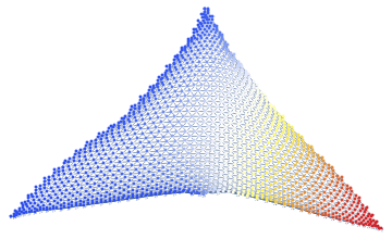
K=GraphGenerator[ResourceFunction["WolframModel"][{{x,y,y},{z,x,u}}{{y,v,y},{y,z,v},{u,v,v}},{{0,0,0},{0,0,0}},1023,"FinalState"]]
Out[]=
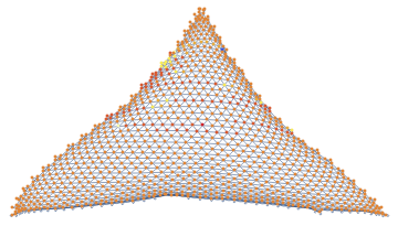
With the graph generated, we define a matrix of initial values to be assigned to each vertex of the graph. We then choose a set of vertices and assign a different value to them, this is done so we can model how shock wave behaves on the generated meshes:
VVals=First[Table[1,{i,32},{j,32}]//MatrixForm]UVals=First[Table[1,{i,32},{j,32}]//MatrixForm]VVals[[(3);;(11),(3);;11]]=Table[ConstantArray[2,9],{i,1,9}]UVals[[(3);;(11),(3);;11]]=Table[ConstantArray[2,9],{i,1,9}]GT1=Graph[K,VertexWeight(VVals//Flatten)]GraphList2={SetProperty[GT1,{VertexStyleThread[VertexList[GT1](ColorData["TemperatureMap"]/@Rescale[VVals//Flatten])]}]}Flatten[GraphList2]
Out[]=
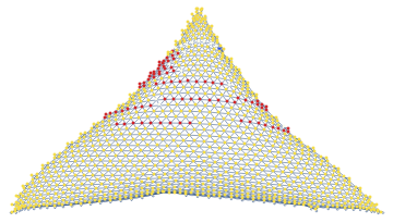
The generated graph has a few values that are higher than the rest of the graph. We will now solve the Burger's Equation and see how this propagates throughout the graph:
dx=0.01dy=0.01dt=0.01For[i=1,i<6,i++,Un=UVals;Vn=VVals;UVals[[2;;31,2;;31]]=(Un[[2;;31,2;;31]]-(dt/dx)*Un[[2;;31,2;;31]]*(Un[[2;;31,2;;31]]-Un[[2;;31,1;;30]])-(dt/dy)*Vn[[2;;31,2;;31]]*(Un[[2;;31,2;;31]]-Un[[1;;30,2;;31]])+(0.01*((dt/dx)^2))*(Un[[2;;31,3;;32]]-(2*Un[[2;;31,2;;31]]+Un[[2;;31,1;;30]]))+(0.01*((dt/dy)^2))*(Un[[3;;32,2;;31]]-(2*Un[[2;;31,2;;31]])+Un[[1;;30,2;;31]]));VVals[[2;;31,2;;31]]=(Vn[[2;;31,2;;31]]-(dt/dx)*Un[[2;;31,2;;31]]*(Vn[[2;;31,2;;31]]-Vn[[2;;31,1;;30]])-(dt/dy)*Vn[[2;;31,2;;31]]*(Vn[[2;;31,2;;31]]-Vn[[1;;30,2;;31]])+(0.01*((dt/dx)^2))*(Vn[[2;;31,3;;32]]-(2*Vn[[2;;31,2;;31]]+Vn[[2;;31,1;;30]]))+(0.01*((dt/dy)^2))*(Vn[[3;;32,2;;31]]-(2*Vn[[2;;31,2;;31]])+Vn[[1;;30,2;;31]]));WGraph=Graph[K,VertexWeight(VVals//Flatten)];GraphList2={GraphList2,SetProperty[WGraph,{VertexStyleThread[VertexList[WGraph](ColorData["TemperatureMap"]/@Rescale[VVals//Flatten])]}]}]Flatten[GraphList2]
Out[]=
,

,
,
,

,
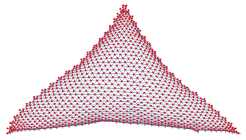

We can see that the model actually does capture shock as we can see the values propagate throughout the system.
From this short demonstration, we established that the Wolfram model meshes, as spatial discretizations, prove to be feasible meshes to solve PDEs numerically on. From here, I think the goal is to try to expand this to more equations and see how the solutions behave on the graphs.
From this short demonstration, we established that the Wolfram model meshes, as spatial discretizations, prove to be feasible meshes to solve PDEs numerically on. From here, I think the goal is to try to expand this to more equations and see how the solutions behave on the graphs.