Artificial life and genes? different way to define cellular automata rules
by Rodrigo A. Obando, Ph.D.
Columbus State University
by Rodrigo A. Obando, Ph.D.
Columbus State University
We introduce a different way to express the one-dimensional cellular automata rules. Instead of using an integer representing the function used to define the rule, we compute a k-dimensional integer vector to represent each rule. Each dimension is defined by the function that determines the behavior of the rule when the state of the cell is of the value of that dimension. These dimensions are labeled ‘genes.’ For instance, for k = 2, each rule is defined by a vector {g0, g1} where g0 is the integer that represents the function (gene) when the cell is 0 and g1 is the integer that represents the function (gene) when the cell is 1. This definition allows for a more structured exploration of the rule spaces, instead of viewing the spaces as ordered lists of integers where the position of the rule is not connected at all to its behavior. In turn, this different arrangement of the rules shows how a particular gene function in the vector may influence the global behavior of a set of rules regardless of the value of other gene, i.e., preserving certain characteristics defined by that common gene. The approach is applicable to cellular automata of any value k.
Introduction
Introduction
We have used Cellular Automata to explore many areas in Science. This simple model serves as a good starting point to investigate many a process or system. Many researchers discover Cellular Automata rules that simulate or model particular behaviors and they have proven to be useful. We hear about particularly interesting rules such as 110 and 30 in the Elementary Cellular Automata rule space (ECA.) The first one is classified as Class 4 or Complex and the second as Class 3 or Random. There are many others that may no be as interesting but nonetheless they do exist in the same space.
In one-dimensional cellular automata, the size of the space depends on the number k of possible values for a cell and the r number of neighboring cells considered to influence the value of the cell on the next evolution step. The following equation provides the number of rules in a space given a value for k and r.
Computes the total number of rules for a given r and k.
In[]:=
TotalNumberOfRules[r_:1,k_:2]:=k^k^(2r+1)
Table 1.
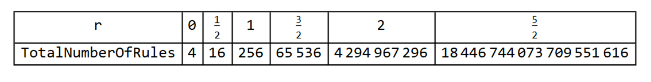
The ECA is the space defined when r = 1. There are just 256 rules and these have been explored and studied throughout the years. If we make r = 3/2, the size of the space is 65536 and this space may not have been explored and studied as much as the ECA due to its size. A value of r = 2 makes the rule space size about 4 billion rules and this space has not been explored either. How do we explore such big spaces? The general view on these spaces is that they do not have a particular structure, that they are a ‘blob.’ Many have defined some schemes but in general they do not provide a suitable way to navigate such spaces in a way that can be applied to all the spaces for different values of r. In fact, the way we normally list the rules in the ECA or any other space is by simply numbering them from 0 to the maximum number minus one. This particular ordering of the rules provides no hint on how the rules relate to each other one way or another. We find that the behavior and the rule numbers have no way of relating similar rules. We can see such listing of the ECA in a New Kind of Science by Wolfram [A] pages 55 and 56. The following figures show the spaces for r = 0 and r = 1/2.
Four colors for coloring evolution class output. Random input to be used with CellularAutomaton
In[]:=
colors=,,,;random=RandomInteger[{0,1},100];
Helper functions to determine class behavior from CellularAutomaton
In[]:=
GetCycles[hist_,numberToDrop_]:=Length[Union[Drop[hist,numberToDrop]]];Classifier[hist_]:=Module[{shifts=Table[RotateRight[hist〚-3〛,n],{n,-5,5}],compare,theClass},compare=Flatten[Position[Table[shifts〚n〛hist〚-1〛,{n,1,Length[shifts]}],True]];If[Length[compare]0,theClass=3,If[MemberQ[compare,6],theClass=1,theClass=2]];theClass];
Computes the class behavior from CellularAutomaton
In[]:=
Detangler[class_,cycles_]:=If[cycles1,1,If[cycles≤512,2,If[class2,class,If[class3&&cycles>512,class,2]]]];ComputeWolframClass[rule_,r_,init_]:=Module[{longHistory=CellularAutomaton[{rule,2,r},init,{1000,All}]},Detangler[Classifier[longHistory],GetCycles[longHistory,50]]];
Figure 1.Rule space for r = 0.
In[]:=
GraphicsGrid[Outer[ArrayPlot[CellularAutomaton[{#2+#12,2,0},{{1},0},{50,{-50,50}}],ColorRules{0White,1colors[[ComputeWolframClass[#2+#12,0,random]]],_Black},PlotLabel#2+#12]&,Range[0,1],Range[0,1]],Frame->True,DividersAll]
Out[]=
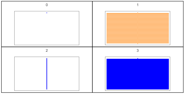
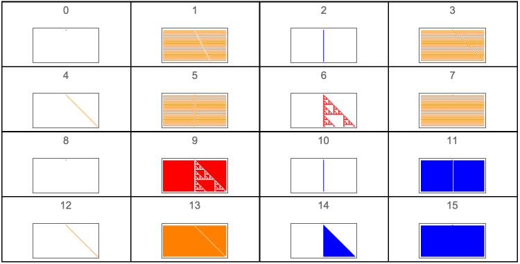
Figure 2.Rule space for r = 1/2.
In[]:=
GraphicsGrid[Outer[ArrayPlot[CellularAutomaton[{#2+#14,2,1/2},{{1},0},{50,{-50,50}}],ColorRules{0White,1colors[[ComputeWolframClass[#2+#14,1/2,random]]],_Black},PlotLabel#2+#14]&,Range[0,3],Range[0,3]],Frame->True,DividersAll]
Out[]=
Rule Genes
Rule Genes
We use the concept of rule gene, first introduced in [B] but under the name of rule primitive, and we split each rule into genes or a gene vector. Each gene does not evolve as a rule but it defines the rule’s behavior given the value of the cell. For k = 2, each rule is split into 2 genes or a 2-dimensional gene vector ({g0, g1}.) The gene in position 0 defines how the cell evolves given that the value of the cell is 0 and the gene in position 1 defines how the cell evolves given that the value of the cell is 1. We may say that each gene gets activated by the value of the cell. A value of 0 activates the gene in position 0 (g0) and a value of 1 activates the gene in position 1 (g1.) Just as the rule number represents an equation or function so do the genes. You may see details in [B].
The number of genes in a rule space are given by TotalNumberOfGenes. We get the genes of a rule using the RuleGenes function, the function FromGenes uses a list of genes to form a rule.
Computes the total number of genes for a given r and k.
In[]:=
TotalNumberOfGenes[r_:1,k_:2]:=k^k^(2r);
Computes a rule number given a gene vector for a given r and k.
In[]:=
FromGenes[genes_,r_:1,k_:2]:=FromDigits[Flatten[Thread[Map[Partition[IntegerDigits[genes[[#]],k,k^(2r)],k^Floor[r]]&,Reverse[Range[k]]]]],k];
Computes the gene vector for a rule for a given r and k.
In[]:=
RuleGenes[rule_,r_:1,k_:2]:=Module[{splitRule=Partition[IntegerDigits[rule,k,k^(2r+1)],k^Floor[r]]},Map[FromDigits[#,k]&,Map[Flatten[splitRule[[Table[n,{n,#,Length[splitRule],k}]]]]&,Reverse[Range[k]]]]];
The following table shows the number of genes for spaces where k = 2.
Table 2.
Out[]=
r | 0 | 1 2 | 1 | 3 2 | 2 | 5 2 |
TotalNumberOfGenes | 2 | 4 | 16 | 256 | 65536 | 4294967296 |
Examples of rules and their genes for r = 1 are shown below.
Table 3.
Out[]=
30 | {6,3} |
23 | {7,1} |
45 | {9,3} |
60 | {12,3} |
90 | {6,6} |
110 | {10,7} |
The following Manipulate lets you enter the rule number to get its genes and you may enter a list of genes and get the rule they form.
Out[]=


We can explore a particular part of the rule space by fixing one of the genes, either at position 0 or position 1, and change the other one. We can make this exploration using the following Manipulates. The first Manipulate uses all 0’s with a single 1 as initial input and the second Manipulate uses all 1’s with a single 0 as initial input.
Manipulate to explore the ECA given a gene at position 0.
In[]:=
Manipulate[GraphicsGrid[Partition[ArrayPlot[CellularAutomaton[{FromGenes[{gene0,#},1,2],2,1},{{1},0},{50,{-50,50}}],ColorRules{0White,1colors[[ComputeWolframClass[FromGenes[{gene0,#},1,2],1,random]]],_Black},PlotLabelToString[FromGenes[{gene0,#},1,2]]<>" - "<>ToString[{gene0,#}]]&/@Range[0,15],4],DividersAll],{{gene0,6,"Gene at position 0"},Range[0,15]},SaveDefinitionsTrue]
Out[]=
Manipulate to explore the ECA given a gene at position 1.
In[]:=
Manipulate[GraphicsGrid[Partition[ArrayPlot[CellularAutomaton[{FromGenes[{#,gene1},1],2,1},{{0},1},{50,{-50,50}}],ColorRules{0White,1colors[[ComputeWolframClass[FromGenes[{#,gene1},1],1,random]]],_Black},PlotLabelToString[FromGenes[{#,gene1},1]]<>" - "<>ToString[{#,gene1}]]&/@Range[0,15],4],DividersAll],{{gene1,9,"Gene at position 1"},Range[0,15]}]
Out[]=
We can arrange the entire rule space by using the outer product of the sets of genes as follows.
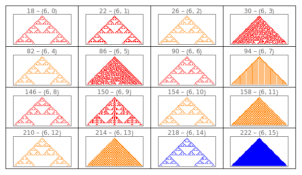
Figure 3.Rule space for r = 1 using the genes. Genes at position 0 for the horizontal and genes at position 1 for the vertical.
In[]:=
GraphicsGrid[Outer[Tooltip[ArrayPlot[CellularAutomaton[{FromGenes[{#2,#1},1],2,1},{{1},0},{50,{-50,50}}],ColorRules{0White,1colors[[ComputeWolframClass[FromGenes[{#2,#1},1],1,random]]],_Black}],FromGenes[{#2,#1},1]]&,Range[0,15],Range[0,15]],Frame->True,DividersAll,ImageSizeLarge]
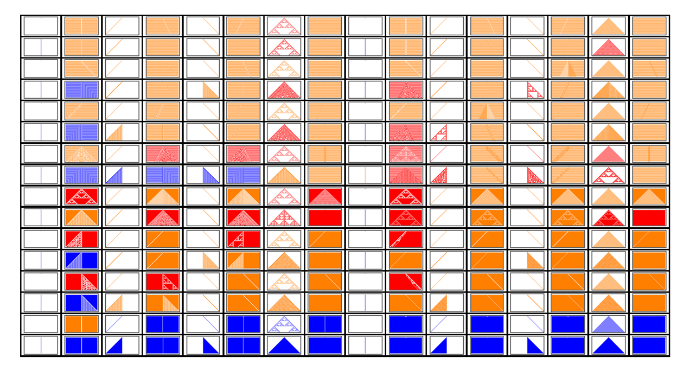
The order used here is simply the natural order for the genes from 0 to 15. The order of the genes defines the general structure of this view. The order used next is developed and provided in detail in [C] and [D]. The list of genes are provided by the following recursive functions. Note: the functions do not work for k > 2. They have this form to later modify them to provide the functionality with the appropriate signature or pattern.
Extends a gene to longer genes by threading or prepending with a gene set
In[]:=
ExtendGene[gene_,r_:1,k_:2]:=Module[{extensions=Map[IntegerDigits[#,k,k^(2r)]&,GeneSet[r,k]]},If[OddQ[2r],Map[FromDigits[Flatten[Thread[{#,IntegerDigits[gene,k,k^(2r)]}]],k]&,extensions],Map[FromDigits[Flatten[Prepend[IntegerDigits[gene,k,k^(2r)],#]],k]&,extensions]]]
Computes a gene set and an offset gene set for a given r and k.
In[]:=
GeneSet[0,k_:2]:=Range[k]-1;GeneSet[r_:1,k_:2]:=GeneSet[r,k]=Flatten[Map[ExtendGene[#,r-1/2,k]&,GeneSet[r-1/2,k]]];OffsetGeneSet[r_:1,k_:2,offset_:1]:=FromDigits[Mod[#+offset,k]&/@Reverse[IntegerDigits[#,k,2^(2r)]],k]&/@GeneSet[r,k];GeneSets[r_:1,k_:2]:=Prepend[OffsetGeneSet[r,k,#]&/@Range[k-1],GeneSet[r,k]];
Using these functions we show the structures of these rule spaces in contrast to how they look in Figures 1 and 2. We are able to see more coherence on the distribution of the rule behavior throughout the rule space. The GeneSet function computes the list of primitives in the particular order presented in [C]. The OffsetGeneSet function computes the conjugate of the GeneSet, preserving the order.
Figure 2.Rule spaces using the GeneSet function.
In[]:=
Manipulate[GraphicsGrid[Outer[Tooltip[ArrayPlot[CellularAutomaton[{FromGenes[{GeneSet[r][[#2+1]],OffsetGeneSet[r][[#1+1]]},r],2,r},If[#2≥#1,init,1-init],{50,{-50,50}}],ColorRules{0White,1colors[[ComputeWolframClass[FromGenes[{GeneSet[r][[#2+1]],OffsetGeneSet[r][[#1+1]]},r],r,random]]],_Black}],FromGenes[{GeneSet[r][[#2+1]],OffsetGeneSet[r][[#1+1]]},r]]&,Range[0,2^2^(2r)-1],Range[0,2^2^(2r)-1]],Frame->True,DividersAll],{r,{0,1/2,1,3/2}},{init,{{{1},0}"Simple",random"Random"}},SaveDefinitionsTrue]
Out[]=
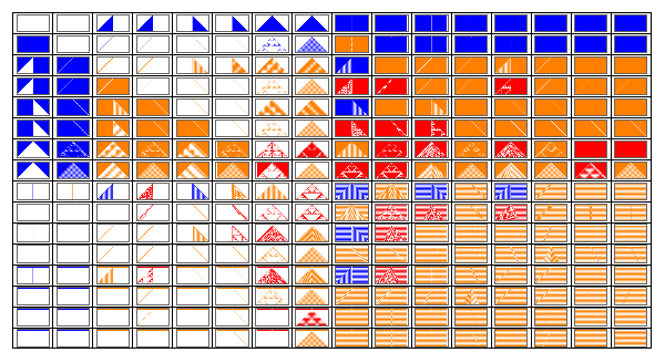
At first glance we may see that the rule behavior distribution seems more coherent. Rules of a particular class are aligned close to each other. The initial conditions change to its conjugate according to where the rule lies in the space; this allows to demonstrate the conjugate symmetry a lot clearly. Also, most Class 1 rules are on a couple of columns/rows in the space. Warning: it will take a long time to compute the output if you select r = 3/2.
Conjugate Symmetry
Conjugate Symmetry
We may observe that the distribution of the rules in this view arranges the conjugate rules (output zeros are output ones and vice-versa) in such a way that they are opposite across the diagonal. For example, for r = 0, rule 0 is the conjugate of rule 3. For r = 1/2, rule 6 is the conjugate of rule 9. This is the same layout regardless of the value of r. The symmetry is along the diagonal. The rules in the diagonal are their own conjugates and the way to show the conjugate behavior is by changing the initial condition to its conjugate. The following Manipulate shows the diagonal of the rule space for different values of r and initial conditions. We may see that by simply conjugating the initial conditions we get the conjugate output generated by the same rule. Again, selecting r = 3/2 will take a long time to compute.
Figure 5.Rule space diagonal.
In[]:=
Manipulate[GraphicsGrid[{Tooltip[ArrayPlot[CellularAutomaton[{#,2,r},init,{50,{-50,50}}],ColorRules{0White,1colors[[ComputeWolframClass[#,r,random]]],_Black}],{#,RuleGenes[#,r,2]}]&/@(FromGenes[#,r]&/@Thread[List[GeneSet[r],OffsetGeneSet[r,2,1]]]),Tooltip[ArrayPlot[CellularAutomaton[{#,2,r},1-init,{50,{-50,50}}],ColorRules{0White,1colors[[ComputeWolframClass[#,r,random]]],_Black}],{#,RuleGenes[#,r,2]}]&/@(FromGenes[#,r]&/@Thread[List[GeneSet[r],OffsetGeneSet[r,2,1]]])}],{r,{0,1/2,1,3/2}},{init,{{{1},0}"Simple",random"Random"}},FrameLabel"Rule Space Diagonal",SaveDefinitionsTrue]
Out[]=

This conjugate symmetry is a special case of the symmetry presented in [C] for values of k greater than 2 which is defined by a function relation named pseudo-additive equivalence. Nonetheless, the diagonal of the rule space is made out of primitives that are the corresponding pseudo-additive equivalent functions and they create rules that are their own shifted functions. A more thorough explanation is found in [C].
Conclusion
Conclusion
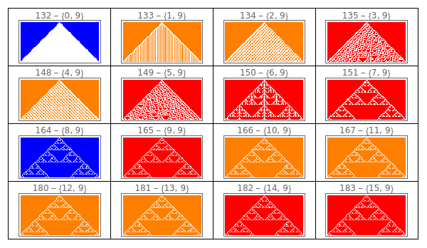
This is a brief introduction to a different way to define the rules, based on simpler function we call genes. We may start using this view and perhaps engineer rules instead of just searching for them in an amorphous space. We may study how a particular gene affects the overall behavior of a set of rules, for instance, you may see how a particular gene defines many of the Sierpinski output for the rules with r = 1 as shown in Figure 4. That particular gene used at position 0 in the rule defines a column with these rules. If we use its conjugate gene in position 1 it defines a row with the conjugate behavior of the rules in the column defined by gene in position 0. This particular gene is the XOR function where its inputs are both neighbor cells; its conjugate is the XNOR function. When we use the gene XOR in position 0 and the gene XNOR in position 1 we get a rule with side-by-side Sierpinski triangles. It is curious to note that these genes are also the ones responsible for the well known class where rule 30 is defined ({30, 86, 135, 149}.)
We also find that the rules and their reflected rules are close to each other; this pattern continues in bigger spaces and is further explored in [C] where it is shown that the reflection symmetry is not global with respect to the space but local. This symmetry defines regions in the space where rules and their corresponding reflections exist.
References
References
[A] Wolfram, Stephen, A New Kind of Science, Champaign, IL: Wolfram Media, 2002.
[B] Obando, Rodrigo, “Partitioning of Cellular Automata Rule Spaces,” Complex Systems, 24, 2015 pp. 27–48.
[C] Obando, Rodrigo, “ On a Unified Model of One-Dimensional Cellular Automata,” Physica D, to be submitted.
[D] Obando, Rodrigo, “Mining and Cataloguing the Computational Universe of Cellular Automata,” in Wolfram Technology Conference (Wolfram Tech Conf 2020), Champaign, Illinois, October 2020, (https://www.wolfram.com/broadcast/video.php?c=488&p=6&v=3317) URL.