Functions
Functions
Functions are a way to assign each point in a chosen domain to one point in a chosen co-domain. Interestingly, the same function can acquire different properties if a different domain and co-domain are chosen. To visualize the effect of choosing a different domain, I will use several WL functions, including Jan Mangaldan's RiemannSphereComplexPlot. [1]
Notation
Notation
Functions, along with (importantly) their chosen domains and co-domains, can be represented using several notations, including the “arrow” and “arrow from bar” notations. [2]
These are all equivalent
f : ℝ→ℝ, f(x) = x²
f : ℝ→ℝ, x ↦ x²
In set theory notation, it is convention to represent some of the most significant sets with double-struck, or “blackboard bold” capital letters (as opposed to ordinary upright Roman letters). Examples: ℕ for natural numbers, ℝ for real numbers, ℂ for complex numbers and so on [3]. I like to use 𝕊 for the Riemann Sphere because it follows this pattern nicely, as the Riemann Sphere is a useful generalization of the complex numbers (ℂ ⊂ 𝕊) the same way complex numbers generalize real numbers and so on.
Furthermore, we can write the image of a set under a function using a square brackets notation [4]. For example, using set builder notation:
f : ℝ→ℝ, f(x) = x²
f[S] = {f(s) | s ∈ S}
f[{1, 2, 3}] = {1, 4, 9}
Injection vs Surjection
Injection vs Surjection
Injections, or “into” or “one-to-one” functions assign each point in their domain to a unique point in their codomain such that no point in the codomain has more than one point in the domain assigned to it. A nice property of them is that they do not have multi-valued inverses. For example, f:ℝ→ℝ=x↦x² is not an injection, so its inverse f⁻¹:ℝ→ℝ,x↦±sqrt(x) is multi-valued. sqrt(4) = 2 and -2. Methods for dealing with multi-valued functions are studied in complex analysis. An example of a function which is injective when you choose the right domain and codomain, however, is f:ℝ→ℝ=x↦x³. You can use InverseFunction[] to find the inverse of a function in WL and test whether it is injective, and Quiet[] to silence the warning message WL gives about multi-valued functions.
In[]:=
#^3&Quiet[ InverseFunction[#^3&] ]Quiet[ InverseFunction[InverseFunction[#^3&]] ]
Out[]=
3
#1
Out[]=
1/3
#1
Out[]=
3
#1
A surjection, also called “onto” or (if it is not also an injection) “many-to-one” is a function whose output maps to the entire co-domain you choose. For example, f:X→Y is a surjection if f[X]=Y. i.e., the image of the domain (the “range”) is equal to the codomain. A function that is not surjective and has missing points in the co-domain is called “partial” whereas a function that has no missing points in the domain is called “total.” The inverse of a surjection might be multi-valued, but it will be total, and have no points in its domain “left out.”
Bijections are the “nicest” kind of function. They are both one-to-one like injections and cover the entire co-domain like surjections. The inverse of a bijection has no points left out and no multi-valued points.
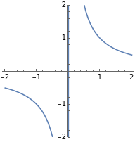
If you ever wondered about division by zero, the Riemann Sphere helps fix this. f:ℝ→ℝ=x↦1/x is not a total function: It has is a missing point in its domain (in this case, a singularity) at x=0. By contrast, f:𝕊→𝕊=z↦1/z is a perfect bijection! It corresponds to rotating the Riemann Sphere 180° around the points z=1 and z=-1.
Bijections are the “nicest” kind of function. They are both one-to-one like injections and cover the entire co-domain like surjections. The inverse of a bijection has no points left out and no multi-valued points.
If you ever wondered about division by zero, the Riemann Sphere helps fix this. f:ℝ→ℝ=x↦1/x is not a total function: It has is a missing point in its domain (in this case, a singularity) at x=0. By contrast, f:𝕊→𝕊=z↦1/z is a perfect bijection! It corresponds to rotating the Riemann Sphere 180° around the points z=1 and z=-1.
Plots showing 1) f using the real numbers as the domain, 2) f using the Riemann Sphere as the domain, and 3) the identity function on the Riemann Sphere, showing how, by comparison, f rotates it 180°. Riemann Sphere plots were generated using Jan Mangaldan’s WFR function “RiemannSphereComplexPlot.”
In[]:=
f[x_]:=1/xGrid[{{Plot[f[x],{x,-2,2},PlotRange2, AspectRatio1],ResourceFunction["RiemannSphereComplexPlot"][f[z], z,ColorFunction->"CyclicReImLogAbs"],ResourceFunction["RiemannSphereComplexPlot"][z, z,ColorFunction->"CyclicReImLogAbs"]}}]
Out[]=
 |  |
So if 1/0 is not undefined on the Riemann Sphere, than what is it?
In[]:=
Quiet[ 1/0 ]
Out[]=
ComplexInfinity
Rotating the Riemann Sphere 180° put its north pole where 0 previously was! This north pole is often called ∞ or complex infinity in complex analysis. WL lets you work with it just like ordinary real numbers or complex numbers!
In[]:=
Quiet[1/(1/0)]
Out[]=
0
Involutions, Trivolutions, Projections, Identities
Involutions, Trivolutions, Projections, Identities
There are many more types of functions, and among the most interesting are involutions and projections.
An identity is a function such that f(x)=x. An involution is a function f:X→X such that f(x)=f⁻¹(x), or, equivalently, f(f(x))=x. A projection is a function f:X→Y such that f(f(x))=f(x). A trivolution is a function f:X→X such that f(f(f(x)))=x.
An identity is a function such that f(x)=x. An involution is a function f:X→X such that f(x)=f⁻¹(x), or, equivalently, f(f(x))=x. A projection is a function f:X→Y such that f(f(x))=f(x). A trivolution is a function f:X→X such that f(f(f(x)))=x.
◼
Every identity is also an involution, a trivolution, and a projection. Every point in the domain of an identity may be considered to be a fixed point under that function, or equivalently, a periodic point of period 1.
◼
A counter-intuitive example of an identity function is f:ℕ→ℕ,n↦floor(n) which is an identity if the domain and range are integers, but not real numbers as in f:ℝ→ℝ,x↦floor(x). floor(2)=2 but floor(2.5)≠2.5
◼
An involution may be considered to be a “half-iterate” of an identity function. A half-iterate of a function g(x) is a function f(x) such that f(f(x))=g(x). Equivalently, every point in the domain of an involution is a periodic point of period 2 under that function.
◼
There are many kinds of projections, ranging from the familiar 3D→2D perspective projection f:ℝ³→ℝ² (where denotes the n-ary Cartesian power) to Stereographic projection f:ℝ²→S² (where denotes the n-sphere ) to taking the components (or “shadows”) of vectors, to taking the real parts of complex numbers, to more familiar ones like multiplication by zero f:ℝ→ℝ,x↦0
n
ℝ
n
S
p+++...=1
2
p
x
2
p
y
2
p
z
◼
All projections f:X→Y have the property that g(x)=f(f(x)) is an identity, and that all points in the image of its domain f[X] are fixed points under f. ∀x∈f[X],f(x)=x.
◼
You can artificially “construct” involutions and trivolutions from injections combined with other involutions and trivolutions. If g:X→Y is an injection, and h:Y→Y is a trivolution, then g⁻¹(h(g(x)) is also a trivolution. For example, h(x) might be a rotation by 120°, or a reflection about some axis in Y.
◼
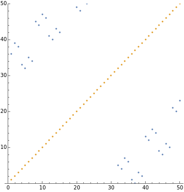
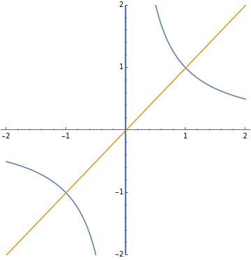
You can tell apart an involution’s plot because it has mirror symmetry around the line y=x. Some examples of involutions are f:ℝ→ℝ,f(x)=x and f:ℝ→ℝ,x↦1/x and f:ℕ→ℕ,n↦n XOR k for some constant integer k.
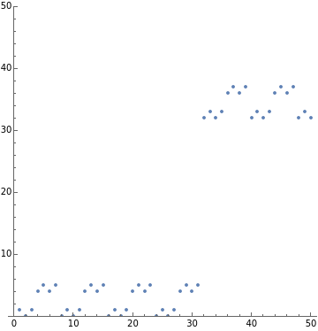
Let’s draw some involutions and projections! Bitwise XOR with a whole number is an involution on the natural numbers, and you can see this by looking at how its graph has perfect mirror symmetry over the line y=x. Furthermore, when it is called twice on itself, it gives x, i.e. BitXor[37, BitXor[37, n]] = n.
f(x)=1/x is another involution, this one works on the set of all Real numbers.
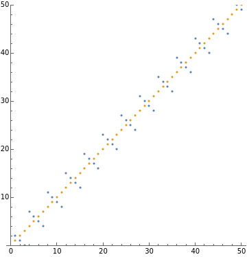
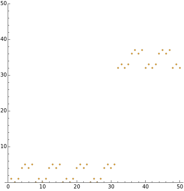
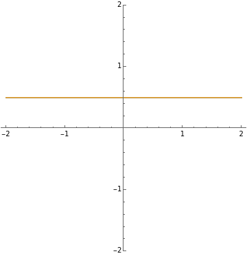
Bitwise AND is a projection. You can see that calling it twice generates the same output as calling it once.
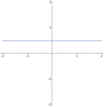
g:ℝ→ℝ,g(x)=0.5+0x or, equivalently, g:ℝ→ℝ,x↦0.5, is an example of a projection. Multiplication by zero is related to taking coordinates of vectors and computing shadows of shapes.
f(x)=1/x is another involution, this one works on the set of all Real numbers.
Bitwise AND is a projection. You can see that calling it twice generates the same output as calling it once.
g:ℝ→ℝ,g(x)=0.5+0x or, equivalently, g:ℝ→ℝ,x↦0.5, is an example of a projection. Multiplication by zero is related to taking coordinates of vectors and computing shadows of shapes.
f[n_]:=BitXor[n,37]g[n_]:=BitXor[n,3]h[x_]:=1/xplotRange=50;(* Injections *)Grid[{{ListPlot[{Table[f[n],{n,1,plotRange}],Table[f[f[n]],{n,1,plotRange}]},PlotRangeplotRange,AspectRatio1],ListPlot[{Table[g[n],{n,1,plotRange}],Table[g[g[n]],{n,1,plotRange}]},PlotRangeplotRange,AspectRatio1],Plot[{h[x],h[h[x]]},{x,-2,2},PlotRange2, AspectRatio1]}}](* Projections f(f(x))=f(x) *)f[n_]:=BitAnd[n,37]g[x_]:=0.5+0*xGrid[{{ListPlot[Table[f[n],{n,1,plotRange}],PlotRangeplotRange,AspectRatio1],ListPlot[{Table[f[n],{n,1,plotRange}],Table[f[f[n]],{n,1,plotRange}]},PlotRangeplotRange,AspectRatio1],Plot[g[x],{x,-2,2},PlotRange2, AspectRatio1],Plot[{g[x],g[g[x]]},{x,-2,2},PlotRange2, AspectRatio1]}}]
Out[]=
Out[]=
References
References
CITE THIS NOTEBOOK
CITE THIS NOTEBOOK
Surjections, projections, involutions, and other classifications of functions
by Chase Marangu
Wolfram Community, STAFF PICKS, August 1, 2023
https://community.wolfram.com/groups/-/m/t/2980863
by Chase Marangu
Wolfram Community, STAFF PICKS, August 1, 2023
https://community.wolfram.com/groups/-/m/t/2980863