Introduction to the problem
Introduction to the problem
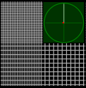
The cover GIF is a rasterized version of Graphics with a bunch of usual primitives. They are designed to be exactly 1 pixel width and is intended to align perfectly with your monitor’s pixels at a specific ImageSize (here the first and last frame of the GIF). One frame of the graphics is included below, can you (especially for readers on Windows) find the correct ImageSize value for Show, so the grids align with pixels on your own screen?
Show
,ImageSize->{width,height}
Pixel based screen is one of the most common media when working with vector graphics. Pixel-perfection is essential when doing digital design, UI composition, etc. However, the computer world (or for sake of this post, the modern Windows desktop world) has a lot of units to measure length, some are related to physical units, many aren’t. These units have confused people (including me) for a long time. A recent question on the sister site, Why AbsoluteThickness depends on ImageSize?, motivated me to finally investigate the topic and get the concepts straight for good and for all. Now that I believe I have a correct understanding of the problem, I think it’s really worth sharing my findings as a tech note. Hopefully it can help other confused fellows to find their own ways to work with vector graphics in a pixel perfect way.
Helper functions
Helper functions
ClearAll[pipe,pipeList,branch,branchSeq]pipe=RightComposition;branch=Through@*{##}&;branchSeq=pipe[branch@##,Apply@Sequence]&;pipeList=pipe[Fold[branchSeq[Identity,pipe[#2,#1]]&,Identity,Reverse@{##}],List]&;
myRasterize is a modified version of Rasterize, so it works correctly for small raster size:
In[]:=
ClearAll[myRasterize]Options[myRasterize]=BackgroundRGBColor,,;myRasterize[graph_Graphics,RasterSizew_Integer,OptionsPattern[]]:=Block[{System`ConvertersDump`createExportPacketExpr,bg=OptionValue[Background]},System`ConvertersDump`createExportPacketExpr[expr_,opts___]:=System`ConvertersDump`createGraphicExportPacketExpr[expr,opts]//Block[{GraphicsBox=Inactive[GraphicsBox]},#/.(BackgroundNone):>Sequence[]]&//Activate;Rasterize[graph,RasterSizew,Backgroundbg]//pipe[RemoveAlphaChannel,ImageData[#,"Byte"]&,DeleteCases[{ImageData[Image[{{bg}}],"Byte",InterleavingTrue][[1,1]]..}],Image[#,"Byte",ColorSpace"RGB"]&]]
93
255
107
255
255
255
Usage:
Graphics[{},BackgroundBlack,ImageSize{10,5}]//pipe[branch[Rasterize[#,RasterSize10]&,myRasterize[#,RasterSize10]&],branch[Identity,Map@ImageDimensions],Prepend[{"Rasterize","myRasterize"}],Transpose,Grid]
Out[]=
Rasterize | {10,16} | |
myRasterize | {10,5} |
All the units in the world
All the units in the world
The inch is not an inch!
The inch is not an inch!
When talking about length on screen, people use inch a lot. Then there are concepts like DPI or dot per inch, PPI or pixel per inch, etc. When I measure my monitor, it’s width with in horizontal. It seems, by “definition” its PPI is
34.4cm
1920px
In[]:=
Quantity[1920,"Pixels"]
UnitConvert[Quantity[34.4,"Centimeters"],"Inches"]
Out[]=
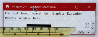
Right? Now, according to the documentation of ImageSize, Wolfram Language uses print’s point for it and assumes per inch. My notebook Magnification is , so ImageSize 72 should give me a graphic exactly wide (i.e. ), right?
72pt
100
%
1inch
2.54cm
In[]:=
CurrentValue[Magnification]Graphics{},BackgroundBlack,AspectRatio,ImageSize72
1
10
Out[]=
1.
Out[]=
Apparently I’m wrong! It’s around :
2.15cm
What is happening? I failed to see a connection between and . That was the first roadblock on my quest.
2.54cm
2.15cm
After some searching and reading, it turned out (see MSDN reference at the end of the post) that on modern Windows desktop, the inch in DPI/PPI is called logical inch, which has nothing to do with the actual inch, and usually does not equate to an actual inch either.
Firstly, the printer’s point (or pt for short), more officially known as desktop publishing point, is an abstract length unit:
In[]:=
Quantity[1,"PrintersPoints"]//{#,#//QuantityUnit}&
Out[]=
,DesktopPublishingPoints
Windows introduced the concept of logical inch (), as I understand it, for compatibility, so this always holds:
in
logic
72pt196px
in
logic
Quote MSDN: “For many years, Windows used the following conversion: One logical inch equals 96 pixels.”
The dot is actually a pixel!
The dot is actually a pixel!
Having understood the logical inch, I can confidently say: Hey! My monitor is working at ! But what about DPI? If the inch is to logical inch, the point is a logical point, what is the dot in DPI?
96PPI
I went out and did some more research. A lot of materials came up, many of them emphasized the difference between DPI and PPI. Unfortunately, that was one of the source of my original confusion, because they are talking about other DPI meanings! Here, for Windows desktop, the dot in DPI IS the same as pixel! Quoting MSDN:
This scaling factor is described as 96 dots per inch (DPI). The term dots derives from printing, where physical dots of ink are put onto paper. For computer displays, it would be more accurate to say 96 pixels per logical inch, but the term DPI has stuck.
But the pixel is not a pixel!
But the pixel is not a pixel!
Okay... but wait! If , why is this Graphics wide instead of ?
72pt96px
120px
96px
In[]:=
Graphics{},BackgroundBlack,AspectRatio,ImageSize72
1
10
Out[]=
In[]:=
(*FromWindows'PrintScreen:*)
//ImageDimensions

Out[]=
{120,12}
The story only got stranger as it so happens that Windows Direct2D introduced yet another abstract/logical layer. The pixel or dot in relation , is something called device-independent pixel or DIP for short. It relates with the actual pixel size ( for short) on physical monitors through Windows DPI scaling factor , which is on my main display:
196px
in
logic
px
λ
DPI
1.25
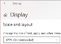
Simply put, Windows aligns with on my monitor. Indeed, ! The same information can also be confirmed from SystemInformation:
100DIP
125px
96DIP×1.25px/DIP120px
In[]:=
SystemInformation["Devices","ConnectedDisplays"]//Lookup["Resolution"]//First
Out[]=
120.
Without diving deeper into the rabbit hole, it’s worth noting that there is still at least one extra layer between DIP and physical pixels: In cases the monitor is not working at native resolution (so the whole desktop and UI could look fuzzy), we’ll have to differentiate rendering pixels () from physical pixels (). For example:
px
rend
px
phy
A monitor with is used, but a non-native resolution is set. Then there will be area unused both at left and right, and a region at center will be re-mapped to for actual display. It means in that case , so physical pixel alignments can happen only at a few certain pixels.
1920×1080
px
phy
px
phy
1440×900
px
rend
px
rend
96×1080
px
phy
px
phy
1728×1080
px
phy
px
phy
1440×900
px
rend
px
rend
56
px
rend
px
phy
In this post, I shall assume native resolution are used, so ≡. Thus without differentiating them, is used afterwards for simplicity.
px
phy
px
rend
px
Wrap-up
Wrap-up
In summary, I now have encountered the following units and concepts: (Really a lot for a seemly simple problem!)
in | Ordinaryrealworldinch |
in logic | Logicalinch,noconnectionwithordinaryin |
pt | Desktoppublishingpoint |
dot | Device-independentpixel,alsoshortformDIPs |
DPI | dotsper in logic |
λ DPI | WindowsDPIscalingsetting |
px rend | “Renderingpixel”asreferredinOS’screenresolutionsettings |
px phy | Physicalpixelasonphysicaldisplays |
They relate to each other by:
72pt196dot≡96DIPs96
in
logic
λ
DPI
px
rend
Again, it is good to confirm my findings through SystemInformation:
SystemInformation["Devices","ConnectedDisplays"]//pipeMap@Association,Map#FullRegion//pipe[Map[Quantity[#,"DesktopPublishingPoints"]&,#,{2}]&,Row[{"[",#1,",",#2,"]"}]&@@@#&,Apply@Inactive[Times]],#FullRegion#Scale//pipe[Map[Quantity[#,IndependentUnit["px"]]&,#,{2}]&,Row[{"[",#1,",",#2,"]"}]&@@@#&,Apply@Inactive[Times]],#Resolution//Quantity#,&,Quantity[1,IndependentUnit[""]]Quantity,"DesktopPublishingPoints"&,MapIndexed[Join[StringTemplate["Display ``"]/@#2,#1]&,#,1]&,Prepend@{"","Region in pt","Region in px","Resolution","pt ⟺ px"},Grid[#,FrameAll,Alignment{Center,Center}]&
IndependentUnit["px"]
IndependentUnit[""]
in
logic
px
rend
1
#Scale
Out[]=
Display 1 | Display 2 | |
Region in pt | [ | [ |
Region in px | [ | [ |
Resolution | ||
pt ⟺ px |
Drawing Graphics pixel-perfectly
Drawing Graphics pixel-perfectly
Pixel alignment and anti-aliasing
Pixel alignment and anti-aliasing
In Wolfram Language’s local Notebook environment, when a Graphics is rendered, ImageSize can be used to specify its display size in pt. According to my previous conclusion, if I draw a width Graphics, I should see it being rendered exactly wide. AbsoluteThickness uses pt as well, so a vertical line with in the same Graphics should be exactly wide. Will it work? Let me try:
3N/(4)pt
λ
DPI
Npx
AbsoluteThickness[3/(4)]
λ
DPI
1px
ModuleW=5,H,xm=RandomReal[{-10,10}],xM=RandomReal[{20,50}],(*nativeScale==*)nativeScale=SystemInformation["Devices","ConnectedDisplays"]//Lookup["Scale"]//First,Δ(*1px==Δpt*),δ(*W*δ==xM-xm*),Δ=;δ=;Graphics[{White,AbsoluteThickness[Δ],Line[{{#,-15},{#,25}}]&@Echo[xm+Echo[2,"Line position in px"]δ,"Line position in Graphics"]},ImageSizeEcho[WΔ,"ImageSize in pt"],PlotRangeEcho[{{xm,xM},{-10,20}},"PlotRange"],PlotRangePaddingNone,BackgroundBlack]
4
3
λ
DPI
1
nativeScale
xM-xm
W
»
Line position in px2
»
Line position in Graphics11.9641
»
ImageSize in pt3.
»
PlotRange{{-5.53469,38.2124},{-10,20}}
Out[]=
Success! It looks like a pixel-perfect alignment is achieved (note 244 in first row is due to anti-aliasing):
In[]:=
(*FromWindows'PrintScreen:*)
//ImageData[#,"Byte",InterleavingTrue]&//Grid[#,FrameAll]&
Out[]=
{0,0,0} | {0,0,0} | {244,244,244} | {0,0,0} | {0,0,0} |
{0,0,0} | {0,0,0} | {255,255,255} | {0,0,0} | {0,0,0} |
{0,0,0} | {0,0,0} | {255,255,255} | {0,0,0} | {0,0,0} |
{0,0,0} | {0,0,0} | {255,255,255} | {0,0,0} | {0,0,0} |
{0,0,0} | {0,0,0} | {255,255,255} | {0,0,0} | {0,0,0} |
By varying the horizontal position (i.e. xpos) of the testing line, I was able to identify the linear relationship between pixel coordinate and Graphics coordinate:
Modulexm=0,xM=20,ym=0,yM=4,W=10,H,(*nativeScale==*)nativeScale=SystemInformation["Devices","ConnectedDisplays"]//Lookup["Scale"]//First,imgsize(*imagesizeinpt*),Δ(*1px==Δpt*),δ(*W*δ==xM-xm*),Δ=;δ=;H=//Ceiling;yM=ym+Hδ;Echo[{{xm,xM},{ym,yM}},"plot range"];imgsize=Echo[Echo[{W,H},"image size in px"]Δ,"image size in pt"];Function[xpos,Graphics[{White,AbsoluteThickness[Δ],Line[{{#,ym-(H-1)δ},{#,yM+(H-1)δ}}]&[xm+xposδ]},ImageSizeimgsize,PlotRange{{xm,xM},{ym,yM}},PlotRangePaddingNone,BackgroundBlack]//pipe[myRasterize[#,RasterSize->W]&(*<-generatea10×2rasterimagehere.*),{Line[{{#,ym-(H-1)δ},{#,yM+(H-1)δ}}]&[xm+xposδ]//InputForm,Item[#,ItemSize{Full,2},AlignmentCenter,BackgroundDarker[Green,.5],FrameTrue,FrameStyleDirective[Thick,Darker[Green,.5]]]}&]]/@Range0,2,(*Subdivide[-1,W,4(W+1)][[;;3]]*)//pipe[Prepend[Item[Style[#,Bold]]&/@{"Line","Rendering result"}],Grid[#,FrameAll]&]
4
3
λ
DPI
1
nativeScale
xM-xm
W
yM-ym
δ
1
4
»
plot range{{0,20},{0,4}}
»
image size in px{10,2}
»
image size in pt{6.,1.2}
Out[]=
Line | Rendering result |
Line[{{0,-2},{0,6}}] | |
Line[{{1/2,-2},{1/2,6}}] | |
Line[{{1,-2},{1,6}}] | |
Line[{{3/2,-2},{3/2,6}}] | |
Line[{{2,-2},{2,6}}] | |
Line[{{5/2,-2},{5/2,6}}] | |
Line[{{3,-2},{3,6}}] | |
Line[{{7/2,-2},{7/2,6}}] | |
Line[{{4,-2},{4,6}}] |


I scanned the test for all and assembled their first row to get the following result:
xpos∈Subdivide[-1,W,4(W+1)]
In[]:=
Module{W=10,xm=0,xM=20,δ},δ=;
xM-xm
W
//pipe[ImageData[#,"Real",InterleavingFalse]&,#[[1]]&,Map[{Subdivide[-1,W,4(W+1)]//xm+#δ&,#}&],ListLinePlot[#,MeshAll,GridLines{{xm,xM},{0,.5,1}},FrameTrue,AxesFalse,FrameLabel{"x in Line[{{x,…},{x,…}}]","pixel value"},PlotLegendsMap[StringTemplate["pixel ``"],Range[W]]]&]
Out[]=
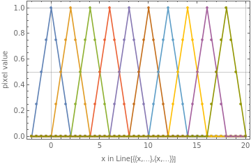
Clearly correspond exactly to pixels to . So it’s a map from (i.e. ) to ∈[1,W]. I especially noted the endpoint of the interval () is NOT included in rendering region!
x∈{+(k-1)δ|k=1,…,W}δ:=-
x
m
x
M
x
m
W
1
W
x∈[,+(W-1)δ]
x
m
x
m
x∈[,-δ]
x
m
x
M
pos
px
x=
x
M
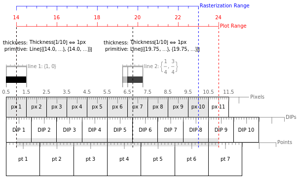
Moreover, the test clearly indicates a simple linear anti-aliasing stage. That means pixel value is proportional with fraction of the pixel area covered by graphic primitive.
Take =14,=24,W=10 for example, the whole affair can be summarized in a single diagram (assume is the left most pixel of the monitor, so px, DIP and pt align at start):
x
m
x
M
px
1
I did a quick check to make sure that is consistent with what I saw directly from my monitor:
Modulexm=14,xM=24,ym=0,yM=4,W=10,H,(*nativeScale==*)nativeScale=SystemInformation["Devices","ConnectedDisplays"]//Lookup["Scale"]//First,imgsize(*imagesizeinpt*),Δ(*1px==Δpt*),δ(*W*δ==xM-xm*),Δ=;δ=;H=//Ceiling;yM=ym+Hδ;Echo[{{xm,xM},{ym,yM}},"plot range"];imgsize=Echo[Echo[{W,H},"image size in px"]Δ,"image size in pt"];GraphicsWhite,AbsoluteThickness[Δ],LineFunction[xpos,{{#,ym-(H-1)δ},{#,yM+(H-1)δ}}&[xm+(xpos-1)δ]]/@1,6+,ImageSizeimgsize,PlotRange{{xm,xM},{ym,yM}},PlotRangePaddingNone,BackgroundBlack//ToBoxes//Cell[BoxData@#,"Output",BackgroundDarker[Green,.5],CellMargins{{300Δ,0},{0,0}},CellFrameMargins{{50Δ,0},{0,0}}]&//CellPrint
4
3
λ
DPI
1
nativeScale
xM-xm
W
yM-ym
δ
3
4
»
plot range{{14,24},{0,4}}
»
image size in px{10,4}
»
image size in pt{6.,2.4}
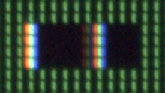
Note Round[255*{1/4, 3/4}] is exactly {64,191}:
Image fromPrintSceen: | Magnified ×20: | Pixel values: | |||||||||||||||||||||||||||||||||||||||||||||||||||||||
| |||||||||||||||||||||||||||||||||||||||||||||||||||||||||
A photo of thescreen region: | |||||||||||||||||||||||||||||||||||||||||||||||||||||||||


Margins -- a hidden pitfall
Margins -- a hidden pitfall
Careful readers may already noticed my explicit settings on CellMargins and CellFrameMargins in the previous example. It so happens that these two options do affect the final result -- considering that they are both measured in pt, this shouldn’t come out as surprising!
Generally speaking, to place a Graphics, it must be contained in a Cell, which itself is in a Notebook. So parameters determining the Graphics’ position include: the top-left corner of the notebook window, the left and top margins from the Cell to notebook’s boundary, and the left and top margins from the Graphics to Cell’s boundary. They can be specified by WindowMargins, CellMargins and CellFrameMargins respectively. On Windows, a native window’s position is always pixel-aligned, so CellMargins and CellFrameMargins are the only settings I need to worry about. To have a pixel-aligned Graphics, it must first be contained in a cell that has its two margins add up to integral pixels:
Total
MarginsInPx
Left/Top
Cell
MarginsInPt
Left/Top
CellFrame
MarginsInPt
Left/Top
96
λ
DPI
72
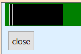
I checked my conclusion with the following example, where a Graphics is shown in a carefully tweaked dark-green Cell in a blue notebook in front of an orange background, with all three kinds of margins controlled:
100px×40px
In[]:=
Modulexm=14,xM=24,ym=0,yM=4(*<-plotrange*),W=100,H(*<-graphicsizeinpx*),wmL=2,wmT=4(*<-WindowMarginsinpx*),cmL=6,cmT=1(*<-CellMarginsinpx*),cfmL=8,cfmT=1(*<-CellFrameMarginsinpx*),(*nativeScale==*)nativeScale=SystemInformation["Devices","ConnectedDisplays"]//Lookup["Scale"]//First,imgsize(*<-imagesizeinpt*),Δ(*1px==Δpt*),δ(*W*δ==xM-xm*),graph,Δ=;δ=;H=//Ceiling;yM=ym+Hδ;Echo[{{xm,xM},{ym,yM}},"plot range"];imgsize=Echo[Echo[{W,H},"image size in px"]Δ,"image size in pt"];graph=GraphicsWhite,AbsoluteThickness[Δ],LineFunction[xpos,{{#,ym-(H-1)δ},{#,yM+(H-1)δ}}&[xm+(xpos-1)δ]]/@1,6+,ImageSizeimgsize,PlotRange{{xm,xM},{ym,yM}},PlotRangePaddingNone,BackgroundBlack;Notebook[{Button["close",NotebookClose[]]//ToBoxes//Cell[BoxData@#,CellMargins100]&},WindowSize{Full,Full},BackgroundLightOrange]//NotebookPut//SelectionMove[#,After,Notebook]&;graph//pipe[ToBoxes,Cell[BoxData@#,"Output",BackgroundDarker[Green,.5],CellMarginsEcho[{{cmL,1},{1,cmT}}Δ,"CellMargins in pt"],CellFrameMarginsEcho[{{cfmL,1},{1,cfmT}}Δ,"CellFrameMargins in pt"],Magnification1]&,Notebook[{#,Button["close",NotebookClose[]]//ToBoxes//Cell[BoxData@#]&},BackgroundLightBlue,WindowFrame"ThinFrame",WindowMargins->Echo[{{wmLΔ,Automatic},{0,wmTΔ}},"WindowMargins in pt"],WindowElements{}]&,NotebookPut,SelectionMove[#,After,Notebook]&];
4
3
λ
DPI
1
nativeScale
xM-xm
W
yM-ym
δ
3
4
»
plot range{{14,24},{0,4}}
»
image size in px{100,40}
»
image size in pt{60.,24.}
»
CellMargins in pt{{3.6,0.6},{0.6,0.6}}
»
CellFrameMargins in pt{{4.8,0.6},{0.6,0.6}}
»
WindowMargins in pt{{1.2,Automatic},{0,2.4}}
A zoom-in of the top-left corner of my screen shows how everything is aligned perfectly:
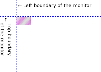
Further zoom-in of the magenta region:
Neat examples
Neat examples
Case 1
Case 1
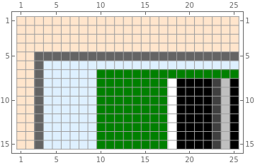
A series of interleaving vertical lines of 1px width:
Module{s,W=100,xm=0,xM=1,nativeScale=SystemInformation["Devices","ConnectedDisplays"]//Lookup["Scale"]//First,Δ,graph,img},Δ=;s=WΔ;graph=GraphicsAbsoluteThickness[Δ],CapForm[None],White,Line{{#,0},{#,.25}}&/@xm+(Range[2,W,2]-1),Red,Line{#,.25},#,.5+&/@xm+(Range[1,W,2]-1),ImageSizes,PlotRange{{xm,xM},{0,.5}},PlotRangePaddingNone,BackgroundBlack;graph//ToBoxes//Cell[BoxData[#],"Output",CellMargins{{30Δ,Inherited},{Inherited,Inherited}},CellFrameMargins{{30Δ,Inherited},{Inherited,Inherited}},BackgroundGray]&//CellPrint
1
nativeScale
xM-xm
W
xM-xm
W
xM-xm
W
zoom-in:
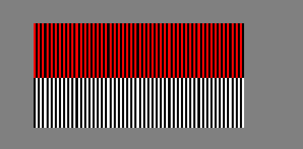
They all align with pixels exactly, so no antialias effect is triggered.
Case 2
Case 2
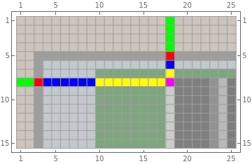
Using AbsoluteThickness is not always desired. Most of the time, fraction based Thickness gives more convenient result, where Thickness[1/W] equals width if the full graphic is rendered with width:
Npx
NWpx
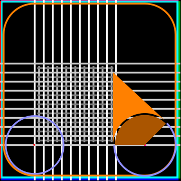
Modulexm=2,xM=6,ym=-1,yM=3(*<-plotrange*),xmpx,ympx,xMpx,yMpx,W=100,H(*<-graphicsizeinpx*),wmL=2,wmT=4(*<-WindowMarginsinpx*),cmL=6,cmT=3(*<-CellMarginsinpx*),cfmL=8,cfmT=3(*<-CellFrameMarginsinpx*),(*nativeScale==*)nativeScale=SystemInformation["Devices","ConnectedDisplays"]//Lookup["Scale"]//First,imgsize(*<-imagesizeinpt*),Δ(*1px==Δpt*),δ(*W*δ==xM-xm*),graph,Δ=;δ=;H=//Ceiling;yM=ym+Hδ;Echo[{{xm,xM},{ym,yM}},"plot range"];imgsize=Echo[Echo[{W,H},"image size in px"]Δ,"image size in pt"];{{xmpx,ympx},{xMpx,yMpx}}={{xm,ym+δ},{xM-δ,yM}};graph=Graphics(*Boundarylines:*)FaceForm[],EdgeFormThickness,Cyan,Rectangle[{xmpx,ympx}+δ,{xMpx,yMpx}-δ],Thickness,CapForm["Square"],Red,Line[{{#,ympx+δ},{#,yMpx-δ}}&@xmpx],Darker[Green],Line[{{#,ympx+δ},{#,yMpx-δ}}&@xMpx],Blue,Line[{{xmpx+δ,#},{xMpx-δ,#}}&@ympx],Lighter[Purple],Line[{{xmpx+δ,#},{xMpx-δ,#}}&@yMpx],(*crossing-pixelgrid:*)Thickness,CapForm["Square"],GrayLevel[0.7],Line[{{#,ympx+21δ},{#,yMpx-37δ}}&/@(xmpx-δ+(Range[20,W-40,5]+2.5)δ)],GrayLevel[0.5],Line[{{xmpx+21δ,#},{xMpx-37δ,#}}&/@(ympx-δ+(Range[20,H-40,5]+2.5)δ)],(*integerpixelgrid:*)Thickness,CapForm["Square"],White,Line[{{#,ympx},{#,yMpx}}&/@(xmpx-δ+Range[20,W-35,5]δ)],GrayLevel[0.8],Line[{{xmpx,#},{xMpx,#}}&/@(ympx-δ+Range[20,H-35,5]δ)],(*Leftcircle:*)Thickness,LighterBlue,,Circle[{xmpx,ympx}-δ+{20,20}δ,(17-1)δ],(*Roundedrectangle:*)FaceForm[],EdgeFormThickness,Orange,Rectangle[{xmpx,ympx}+2δ,{xMpx,yMpx}-2δ,RoundingRadius17δ],(*Rightcircle:*)Thickness,LighterBlue,,CapForm[None],,(*Circlecenters:*)PointSize,Red,Point[{{xmpx,ympx}-δ+{20,20}δ,{xmpx,ympx}-δ+{W-20+1,20}δ}],AbsolutePointSize[Δ],Magenta,Point[{{xmpx,ympx}-δ+{20,20}δ,{xmpx,ympx}-δ+{W-20+1,20}δ}],(*Splineshapes:*)EdgeForm[],FaceForm[Orange],FilledCurve@Line{xmpx,ympx}-δ+{W-20+1,20}δ-17+,0δ,{xmpx,ympx}-δ+{W-20+1,20}δ-17+,0δ+{0,40}δ,,FaceForm[Darker[Orange]],FilledCurve@Line{xmpx,ympx}-δ+{W-20+1,20}δ,{xmpx,ympx}-δ+{W-20+1,20}δ-17-,0δ,,ImageSizeimgsize,PlotRange{{xm,xM},{ym,yM}},PlotRangePaddingNone,BackgroundBlack,BaseStyle->{BSplineCurveBoxOptions->{Method->{"SplinePoints"->100}}}
4
3
λ
DPI
1
nativeScale
xM-xm
W
yM-ym
δ
1
W
1
W
1
W
1
W
1
W
5
9
1
W
1
W
5
9
1
W
1
2
1
2
1
2
»
plot range{{2,6},{-1,3}}
»
image size in px{100,100}
»
image size in pt{60.,60.}
Out[]=

This Graphics was designed to be pixel-perfect when rendered to regardless the displaying monitor. A ×6 zoom-in of the screen shows how it was rendered:
100px×100px
Some key features from my little artwork:
◼
The four boundaries occupy exactly each.
1px
◼
The four corner pixels were left untouched.
◼
The grids aligned with pixels (so they occupy width) or with edges of pixels (so they occupy width).
1px
2px
◼
The left circle touched the rounded rectangle precisely. (Especially comparing with scaled up vector Graphics.)
◼
A gap between two FilledCurve objects was controlled to be precisely width.
1px
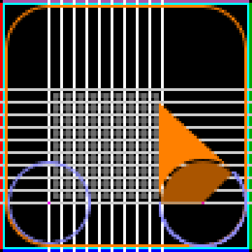
For comparison, this shows a ×6 scale-up of the vector Graphics itself:
References
References