In many engineering and scientific applications, simulating physical systems can be computationally expensive—especially when dealing with complex models governed by differential equations. Surrogate modeling offers a solution by approximating these systems with faster, data-driven alternatives.
One powerful technique for surrogate modeling is the Continuous-Time Echo State Network (CTESN), which combines the expressive power of neural networks with the structure and efficiency of reservoir computing. This method allows us to approximate system behavior with high fidelity and low computation cost.
Use Case—Optimization Speed Enhancements
Use Case—Optimization Speed Enhancements
High-fidelity physical models provide accurate results, but they often come at the cost of significant computation time—especially during iterative tasks like parameter optimization. A Continuous-Time Echo State Network (CTESN)-based surrogate model can drastically reduce optimization time while maintaining sufficient accuracy.
This use case demonstrates how to calibrate a model using both the full physical simulation and the surrogate model, comparing their computational performance and accuracy in an optimization task.
Calibration Using High-Fidelity Model
Calibration Using High-Fidelity Model
We begin by calibrating a detailed physical model using real or synthetic measured data (dataMeasured) and the SystemModelCalibrate function.
In[]:=
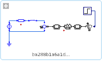
modelPath="DocumentationExamples.Simulation.HybridMotor";dataMeasured=;(*Pre-recordedtimeseriesdata*)(*Calibrateparametersusingactualsimulationmodel*)
In[]:=
AbsoluteTiming[calibratedModel=SystemModelCalibrate[<|"Inertia2.w"->dataMeasured|>,modelPath,{"Resistor1.R","SpringDamper1.d"}]](*Output:{~47seconds,calibratedparametervalues}*)
Out[]=
43.473,
In[]:=
Show[SystemModelPlot[calibratedModel,{"Inertia2.w"},40],ListPlot[dataMeasured,PlotStyle->RGBColor[0.880722,0.611041,0.142051]],PlotRange->All]
Out[]=
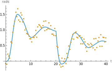
This process is accurate but slow, especially if used in loops or global optimization.\b
Calibration Using Surrogate Model
Calibration Using Surrogate Model
Part 2 — Generate Surrogate Model (CTESN)
Part 2 — Generate Surrogate Model (CTESN)
We now build a surrogate neural network model using the CTESN framework. The surrogate captures the dynamic behavior of the original model for a range of parameters.
In[]:=
(*Definethemodelandparameters*)surrogateModelPath="DocumentationExamples.Simulation.HybridMotor";outputVariables={"Inertia2.w"};simulationDuration=40;nominalParameters={"Resistor1.R"->0.5,"SpringDamper1.d"->0.2};parameterVariation=1.0;(*±100%variation*)reservoirNeurons=100;rbfCentroids=25;(*Trainthesurrogatemodel*)surrogate=CTESNmodel[surrogateModelPath,outputVariables,simulationDuration,<|"ParameterValues"->nominalParameters|>,parameterVariation,reservoirNeurons,rbfCentroids];
Part 3 — Define Surrogate-Based Prediction and Cost Function
Part 3 — Define Surrogate-Based Prediction and Cost Function
Now we define a surrogate-based prediction function and a cost function for optimization.
In[]:=
(*Surrogatepredictionasafunctionofparametersrandd*)ClearAll[predictOutput];predictOutput[r_?NumericQ,d_?NumericQ]:=timeSeriesVar[1,{r,d},surrogate];(*Resampleoriginalmeasureddataforalignment*)referenceOutput=TimeSeriesResample[TimeSeries[dataMeasured],{0,simulationDuration,N[simulationDuration/1999]}];(*Costfunction:squarednormofthedifference*)ClearAll[costFunction];costFunction[r_?NumericQ,d_?NumericQ]:=Norm[Values[referenceOutput]-Values[predictOutput[r,d]]]^2;
Part 4 — Optimize Using Surrogate
Part 4 — Optimize Using Surrogate
We now perform parameter optimization using the fast surrogate model.
In[]:=
(*Globaloptimizationusingdifferentialevolution*)AbsoluteTiming[optimizedParams=NMinimize[{costFunction[r,d],r>0,d>0},{r,d},Method->"DifferentialEvolution",WorkingPrecision->2,AccuracyGoal->2]](*Output:{~6.5seconds,{minimumvalue,optimal{r,d}}}*)
Out[]=
{5.53571,{1.0×,{r0.46,d0.33}}}
2
10
This process is much faster than the original full-model calibration (over 7× speedup in this example).
Part 5 — Visualize the Results
Part 5 — Visualize the Results
In[]:=
Show[ListLinePlot[dataMeasured,PlotStyle->RGBColor[0.880722,0.611041,0.142051]],ListPlot[predictOutput@@Values[optimizedParams[[2]]],PlotStyle->Red],PlotRange->All,PlotLabel->"Comparison: Measured vs. Surrogate Prediction"]
Out[]=
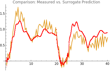
The red curve (surrogate prediction) closely follows the blue curve (measured output), confirming the surrogate model’s fidelity.
Summary
Summary
Out[]=
Step | Full Model | Surrogate Model |
Calibration Time | ~47 seconds | ~6.5 seconds |
Optimization Accuracy | High | High |
Speedup | ~7× faster | |
Usefulness in Optimization | Limited (slow) | Highly efficient |
This demonstrates how CTESN-based surrogate modeling enables fast parameter optimization with minimal loss in accuracy—ideal for use in control loops, design space exploration, and sensitivity studies.
Initialization
Initialization
Building a Surrogate Model Using Continuous-Time Echo State Networks
Building a Surrogate Model Using Continuous-Time Echo State Networks
Introduction
Introduction
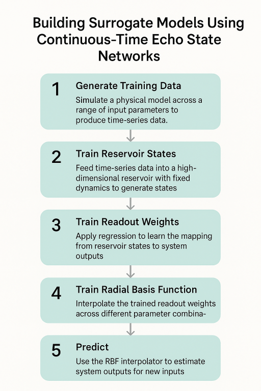
The process of building a CTESN-based surrogate model involves the following five structured steps:
◼
Step 1 — Generate Training Data
We simulate a physical model (e.g., the shaft speed for a DC motor) using a range of input parameters. This produces time-series data that captures the system’s dynamic responses. The simulations use adaptive solvers, and we retain the solver’s raw time steps to preserve temporal accuracy for the next stage.
Step 2 — Train Reservoir States
A randomly chosen simulation output is used to drive a high-dimensional reservoir—a fixed nonlinear system that transforms input signals into rich internal representations. The reservoir states are updated over time using the adaptive time steps, and then interpolated to a uniform time grid.
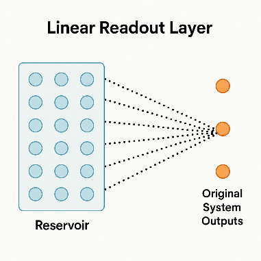
Step 3 — Train Readout Weights
The internal reservoir states are mapped back to the system’s outputs using simple linear regression. This step “trains” the model by learning how to decode the system response from the reservoir’s state at each time step.
Step 4 — Train Radial Basis Function (RBF) Interpolator
To generalize across different parameter combinations, we use an RBF network to interpolate the trained readout weights. This allows the surrogate model to respond to new input parameters by estimating appropriate weights without retraining.
Step 5 — Predict
Given a new parameter set, the RBF interpolator estimates the readout weights, which are then applied to the reservoir states to generate the predicted output signal. This allows for fast, accurate predictions of system behavior—without the need for expensive simulations.
We simulate a physical model (e.g., the shaft speed for a DC motor) using a range of input parameters. This produces time-series data that captures the system’s dynamic responses. The simulations use adaptive solvers, and we retain the solver’s raw time steps to preserve temporal accuracy for the next stage.
Step 2 — Train Reservoir States
A randomly chosen simulation output is used to drive a high-dimensional reservoir—a fixed nonlinear system that transforms input signals into rich internal representations. The reservoir states are updated over time using the adaptive time steps, and then interpolated to a uniform time grid.
Step 3 — Train Readout Weights
The internal reservoir states are mapped back to the system’s outputs using simple linear regression. This step “trains” the model by learning how to decode the system response from the reservoir’s state at each time step.
Step 4 — Train Radial Basis Function (RBF) Interpolator
To generalize across different parameter combinations, we use an RBF network to interpolate the trained readout weights. This allows the surrogate model to respond to new input parameters by estimating appropriate weights without retraining.
Step 5 — Predict
Given a new parameter set, the RBF interpolator estimates the readout weights, which are then applied to the reservoir states to generate the predicted output signal. This allows for fast, accurate predictions of system behavior—without the need for expensive simulations.
Together, these steps enable the creation of an efficient and accurate surrogate model that can replace time-consuming simulations in tasks such as optimization, sensitivity analysis, and real-time control.
Step 1—Generate Training Data
Step 1—Generate Training Data
Objective:
Objective:
Generate time-series data that captures the system’s dynamic behavior for various combinations of input parameters. This data will later be used to train the reservoir in the Continuous-Time Echo State Network.
Key Concepts:
Key Concepts:
◼
System Model: A predefined dynamic model from which data is simulated (e.g., a DC motor model).
◼
Outputs: The variables you want to track over time (e.g., shaft speed).
◼
Parameter Sampling: Varying input parameters within a range to generate diverse training scenarios.
◼
RawData Property: Fetches time series data directly from the solver, retaining its adaptive step sizes—important for accurate temporal modeling.
Example Setup:
Example Setup:
In[]:=
modelName="DocumentationExamples.Simulation.HybridMotor";outputVars={"Inertia2.w"};simTime=40;parameters={"Resistor1.R"->0.5,"SpringDamper1.d"->0.2};(*Nominalparametervalues*)variationParameter=0.5;(*±50%variationaroundnominalvalues*)
◼
simTime: Duration of each simulation (e.g., 40 seconds).
◼
parameters: Nominal input parameters.
◼
variationParameter: Degree of variation from nominal value (±50% in this example).
Data Generation Function:
Data Generation Function:
In[]:=
generateData[model_,variable_,time_,p_,range_]:=Module[{p0,numObservationsTrain,m,M,pTrain,tTrain,yTrain,data,sim1},p0=Values[p["ParameterValues"]];numObservationsTrain=100;(*Createlowerandupperboundsforsampling*)m=(1-range)*p0;M=(1+range)*p0;(*Samplerandomparametersets*)pTrain=Table[m+(M-m)RandomReal[1,Length[M-m]],{numObservationsTrain}];(*Initializeoutputstorage*)tTrain=ConstantArray[0,numObservationsTrain];yTrain=ConstantArray[0,numObservationsTrain];data=ConstantArray[0,numObservationsTrain];(*Runsimulationsinparallel*)sim1=SystemModelSimulate[model,time,<|"ParameterValues"->Thread[Keys[p["ParameterValues"]]->Transpose@pTrain]|>,ProgressReporting->None];(*Extractrawtimeseriesforeachrun*)Table[data[[i]]=sim1[[i]]["RawData",variable];tTrain[[i]]=Transpose[data[[i,1]]][[1]];(*Timevector*)yTrain[[i]]=Transpose[data[[i]][[#]]][[2]]&/@Range[Length[variable]],{i,1,numObservationsTrain}];{tTrain,yTrain,pTrain}];
Run the Data Generation:
Run the Data Generation:
In[]:=
AbsoluteTiming[{timeTraining,outputTraining,parameterTraining}=generateData[modelName,outputVars,simTime,<|"ParameterValues"->parameters|>,variationParameter];]
Out[]=
{10.1018,Null}
◼
This returns a triple of:
◼
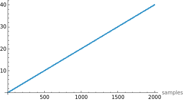
timeTraining: List of time vectors for each run.
◼
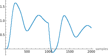
outputTraining: Time series values of output variables.
◼
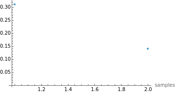
parameterTraining: Parameter values used for each run.
Visualizing the Data:
Visualizing the Data:
In[]:=
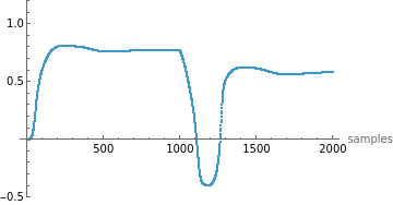
Manipulate[ListPlot[#[[i]],PlotRange->All,AxesLabel->{"samples",Automatic}]&/@{timeTraining,outputTraining,parameterTraining},{i,1,100,1},SaveDefinitions->True]
Out[]=


◼
Use this to inspect how the outputs and time steps vary across simulations.
Why Use “RawData”?
Why Use “RawData”?
Unlike fixed-step solvers, adaptive solvers take smaller steps during rapid changes (e.g., stiff dynamics) and larger steps during slower changes. This produces:
◼
Efficient data capture
◼
More realistic training signals for the CTESN, which benefits from irregular time sampling.
Step 2—Train Reservoir States
Step 2—Train Reservoir States
Objective:
Objective:
Generate the internal reservoir states by projecting simulation output into a high-dimensional dynamical system. These states capture the system’s nonlinear dynamics and serve as features for the final surrogate model.
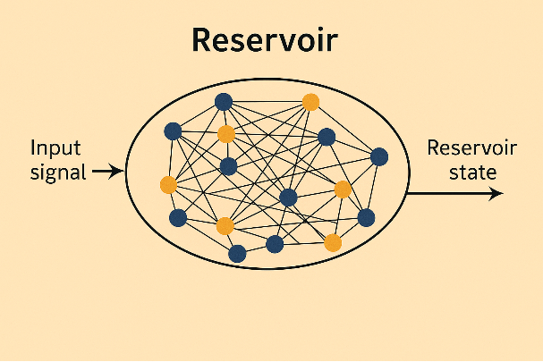
What is a Reservoir?
What is a Reservoir?
A reservoir in an Echo State Network is a fixed, randomly connected dynamical system. It takes input time-series data and transforms it into a rich set of internal states that encapsulate temporal features.
Main Steps:
Main Steps:
1. Set the Reservoir Size
In[]:=
reservoirSize=50;
◼
This sets the dimensionality of the reservoir. Larger sizes can capture more complex dynamics but require more computation.
2. Select a Random Simulation
In[]:=
sampleRandom=RandomInteger[{1,Length[parameterTraining]}];ypStarInterpolant=outputTraining[[sampleRandom]];tpStar=timeTraining[[sampleRandom]];
◼
A random simulation is picked to train the reservoir.
◼
ypStarInterpolant is the time-series output (e.g., shaft speed).
◼
tpStar is the time vector corresponding to that simulation.
3. Generate Reservoir States
In[]:=
AbsoluteTiming[rState=reservoirState[ypStarInterpolant,tpStar,simTime,reservoirSize];]
Out[]=
{0.254357,Null}
◼
This calls the function that evolves reservoir dynamics over the input signal.
In[]:=
reservoirState[ypStarInterpolant_,tpStar_,timeSim_,reservoirSize_]:=Module[{reservoirDims,density,A,V,r0,dr,drTrain,data,rData,rTrainData,timeStepSize,numSimSteps},(*1.Setbasicdimensionsandsparsity*)reservoirDims=reservoirSize;density=0.01;numSimSteps=2000;timeStepSize=timeSim/numSimSteps;(*2.Createsparsesymmetricpositivedefinitematrix*)A=Normal@ResourceFunction["RandomSparseSPDMatrix"][reservoirDims,"CholeskyFactorDensity"->density];(*3.Randominputweights*)V=RandomReal[{0,0.5},{reservoirDims,First@Dimensions[ypStarInterpolant]}];(*4.Initialreservoirstate*)r0=ConstantArray[0,reservoirDims];(*5.Reservoirupdatefunction*)dr[r_,i_]:=Tanh[A.r+V.ypStarInterpolant[[All,i]]];(*6.Timeevolutionofreservoir*)drTrain[r_]:=Module[{length=Length[tpStar],rTrain=ConstantArray[0,Length[tpStar]],rNew=r,time=0},Table[rTrain[[i]]=rNew;rNew=dr[rNew,i],{i,1,length,1}];{tpStar,Join[rTrain,Transpose[{ConstantArray[1,Length[rTrain]]}],2]}];(*7.Interpolatethestates*)data=drTrain[r0];rData=Interpolation[DeleteDuplicatesBy[Transpose[{data[[1]],Transpose[data[[2]]][[#]]}],First],InterpolationOrder->2]&/@Range[reservoirDims+1];(*8.Uniformsamplingofstates*)rTrainData=Table[Through[rData[t]],{t,0,timeSim-timeStepSize,timeStepSize}];rTrainData]
Explanation of Key Concepts:
Explanation of Key Concepts:
◼
Matrix A: A sparse, symmetric, positive-definite matrix that governs internal dynamics. Created using a resource function for numerical stability and efficiency.
◼
Matrix V: Connects the input to the reservoir. Random values introduce variability for learning diverse patterns.
◼
Update Rule: At each timestep, the new reservoir state is:
◼
r (t + 1) = tanh (A ⋅ r (t) + V ⋅ input)
◼
Adaptive Time Input: The state updates align with the solver’s time steps (from RawData), which are often non-uniform.
◼
Interpolation: Since solver time steps are irregular, the states are interpolated and re-sampled at uniform intervals, making them suitable for machine learning.
Visualize Reservoir State Evolution:
Visualize Reservoir State Evolution:
In[]:=
Manipulate[ListPlot[Transpose[rState][[i]],PlotRange->{Automatic,{-0.5,1.2}},AxesLabel->{"samples",Automatic}],{i,1,Length[Transpose[rState]],1},SaveDefinitions->True]
Out[]=
◼
This helps explore how each reservoir neuron evolves in response to the input signal.
Why This Step Matters
Why This Step Matters
This step creates a temporal feature map of the system’s response. It allows a simple model in the next step to linearly read out (or decode) the system dynamics from these rich, nonlinear representations.
Step 3—Train Weights
Step 3—Train Weights
Objective:
Objective:
Train a linear readout layer that maps the high-dimensional reservoir states to the original system output. This is achieved using linear regression, making the final prediction fast and efficient.
Concept Overview:
Concept Overview:
◼
After projecting the original input into a nonlinear high-dimensional space (via the reservoir), the CTESN learns how to decode or read out the original outputs from those transformed features.
◼
The training is done by fitting a set of linear weights (one per output variable) that best map the reservoir states to the true system outputs.
Key Steps:
Key Steps:
1. Uniformly Sample Simulation Output
Simulation outputs were previously generated with adaptive time steps. To match them with reservoir state samples, they are interpolated and resampled at uniform intervals.
Simulation outputs were previously generated with adaptive time steps. To match them with reservoir state samples, they are interpolated and resampled at uniform intervals.
2. Perform Linear Regression
Using the interpolated output data (yData) and the corresponding reservoir states (rTrainData), perform linear regression to find the best weights.
Using the interpolated output data (yData) and the corresponding reservoir states (rTrainData), perform linear regression to find the best weights.
Training Code
Training Code
In[]:=
AbsoluteTiming[resultsData=ParallelTable[weights[rState,outputTraining[[i]],timeTraining[[i]],simTime],{i,1,Length[outputTraining]}];]
Out[]=
{0.195657,Null}
◼
resultsData stores the trained weight matrices for each simulation.
◼
Uses ParallelTable to speed up the training across all simulation samples.
In[]:=
weights[rTrainData_,yInterpolant_,timeTraining_,time_]:=Module[{yData,yData1,Wp,timeStepSize,numSimSteps},numSimSteps=2000;timeStepSize=time/numSimSteps;(*1.Interpolatethesimulationoutput*)yData1=Interpolation[DeleteDuplicatesBy[Transpose[{timeTraining,Transpose[yInterpolant[[#]]]}],First]]&/@Range[First@Dimensions[yInterpolant]];(*2.Resampleoutputatuniformintervals*)yData=Table[Map[yData1[[#]][t]&,Range[First@Dimensions[yInterpolant]]],{t,0,time-timeStepSize,timeStepSize}];(*3.Solvethelinearleastsquaresproblem*)Wp=LeastSquares[rTrainData,yData];Wp];
Explanation of Key Components:
Explanation of Key Components:
◼
rTrainData: The uniformly sampled reservoir states over time.
◼
yInterpolant: The original simulation output for a specific run.
◼
yData: The interpolated and resampled output values.
◼
Wp: The trained linear weights (output layer), calculated by solving:
◼
minimize
∥𝑅⋅𝑊−𝑌
2
∥
◼
where:
◼
R is the matrix of reservoir states,
◼
W is the matrix of weights to solve for,
◼
Y is the actual system output.
Why Linear Regression?
Why Linear Regression?
The reservoir already introduces nonlinearity. A simple linear readout is sufficient to approximate even complex system behaviors, making the model lightweight and fast.
You now have:
◼
A trained reservoir (fixed internal dynamics)
◼
A readout layer (Wp) that maps reservoir states to predicted outputs
Together, these form a surrogate model that can replicate the system’s behavior at a fraction of the simulation cost.
Step 4—Train Radial Basis Function
Step 4—Train Radial Basis Function
Objective:
Objective:
Use a Radial Basis Function (RBF) network to interpolate the trained weights across the parameter space. This enables the surrogate model to predict new system responses for parameter values that were not explicitly simulated.
Why RBF?
Why RBF?
The CTESN builds a model for each training parameter set by learning reservoir-to-output weights. But what if you want to predict the output for new parameter values?
This is where RBF comes in — it acts as a function approximator that maps new parameter values to the corresponding reservoir weights by interpolating between known ones.
Core Idea:
Core Idea:
Think of each set of trained weights (resultsData) as a function of the input parameters (parameterTraining).
Use RBF interpolation to smoothly map from parameters to weights.
Set the Number of Centroids
Set the Number of Centroids
In[]:=
numberOfCentroids=25;
◼
Centroids act like “landmarks” in the parameter space for the interpolation.
◼
More centroids improve accuracy but increase computational cost.
Train the RBF Model
Train the RBF Model
In[]:=
AbsoluteTiming[{W2,centroids,sigma}=trainRBF[parameterTraining,resultsData,numberOfCentroids];]
Out[]=
{0.0064614,Null}
◼
W2: The trained RBF weight tensor.
◼
centroids: Randomly selected parameter points used for interpolation.
◼
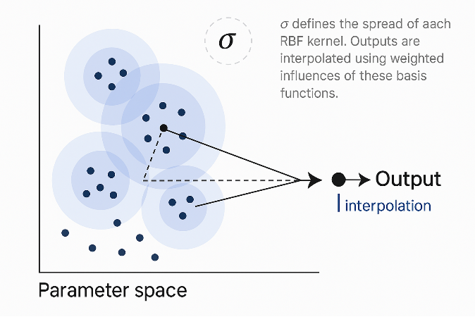
sigma: Controls the smoothness (spread) of each RBF kernel.
Examine Outputs
Examine Outputs
In[]:=
Dimensions[W2]
Out[]=
{26,51,1}
◼
This tells us:
◼
26 basis functions (25 centroids + bias term)
◼
51 reservoir neurons
◼
1 output variables
Centroids (sample) :
Centroids (sample) :
In[]:=
MatrixForm[centroids]
Out[]//MatrixForm=
0.646496 | 0.216305 |
0.36788 | 0.162621 |
0.739779 | 0.16674 |
0.749776 | 0.213984 |
0.619125 | 0.267581 |
0.417048 | 0.136731 |
0.40724 | 0.224774 |
0.745427 | 0.114193 |
0.400881 | 0.200288 |
0.560901 | 0.196719 |
0.479631 | 0.129552 |
0.405749 | 0.142127 |
0.520034 | 0.104086 |
0.528834 | 0.199646 |
0.521955 | 0.274853 |
0.619518 | 0.101489 |
0.635596 | 0.297601 |
0.538886 | 0.101285 |
0.332744 | 0.168921 |
0.330738 | 0.175897 |
0.608308 | 0.280946 |
0.639218 | 0.27991 |
0.579142 | 0.296276 |
0.306818 | 0.106344 |
0.702323 | 0.28266 |
Each row is a parameter vector (e.g., resistance and damping).
Spread Parameter (σ):
Spread Parameter (σ):
In[]:=
sigma
Out[]=
0.069061
Determines how broadly each RBF kernel influences the interpolation.
In[]:=
trainRBF[pTrain_,target_,nCenters_]:=Module[{centroids,distMax,n,sigma,a,a1,U,W2},(*1.Randomlypickcentroids*)centroids=RandomSample[pTrain,nCenters];(*2.Computemaxpairwisedistancebetweencentroids*)distMax=Max[Map[EuclideanDistance[#[[1]],#[[2]]]&,Subsets[centroids,{2}]]];(*3.Computedistancefromeachparameterpointtoeachcentroid*)n=Table[Table[EuclideanDistance[pTrain[[i]],centroids[[j]]],{i,1,Length[pTrain]}],{j,1,Length[centroids]}];(*4.Setσ(kernelspread)*)sigma=distMax/Sqrt[2*nCenters];(*5.DefineRBFactivation*)a[n_]:=Exp[-((n)^2/(2*sigma^2))];a1=a[n];(*6.Createinputmatrixforregression(addbias)*)U=Append[a[n],ConstantArray[1,Length[pTrain]]];(*7.Solveforweightsusingleastsquares*)W2=LeastSquares[U.Transpose[U],U.target];{W2,centroids,sigma}];
Why This Step Matters:
Why This Step Matters:
This step allows the surrogate model to generalize:
◼
You no longer need to simulate the full system for new parameter values.
◼
You simply compute the RBF response for the new parameters and obtain the corresponding reservoir-to-output weights (Wp).
Step 5—Predict
Step 5—Predict
Objective:
Objective:
Use the trained Radial Basis Function (RBF) network and reservoir to predict the system output for new parameter values — without running a full simulation.
Overview:
Overview:
At this point, you have:
◼
Trained reservoir dynamics (rState)
◼
Trained readout weights for known parameters (resultsData)
◼
An RBF interpolation model (W2, centroids, sigma) to map new parameters to readout weights
Now, you use this setup to predict the output for new parameters, like {resistance -> 0.1, damping -> 0.1}.
1. Make a Prediction
1. Make a Prediction
In[]:=
CTESNres=predictRBF[{{0.1,0.1}},centroids,W2,sigma];
◼
Input: A new parameter vector (e.g., resistance and damping).
◼
Output: A predicted readout weight matrix for that parameter setting.
This output is a list of dot-product-ready weights to apply to the reservoir state.
2. Apply the Weights to Reservoir State
2. Apply the Weights to Reservoir State
Now, use the predicted weights to generate the final output signal from the reservoir state:
In[]:=
ListLinePlot[TimeSeries[Transpose[(rState.CTESNres[[1]])][[1]],{0,simTime}],PlotRange->All]
Out[]=
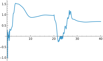
◼
rState: Reservoir states previously computed from a random or test signal.
◼
CTESNres[[1]]: The weight matrix interpolated by RBF for the test parameters.
◼
The dot product rState . weights computes the predicted output over time.
In[]:=
predictRBF[pTest_,centroids_,weights_,sigma_]:=Module[{n,a,U},(*1.Computedistancefromtestpoint(s)toallcentroids*)n=Table[Table[EuclideanDistance[pTest[[i]],centroids[[j]]],{i,1,Length[pTest]}],{j,1,Length[centroids]}];(*2.Defineradialbasisfunctionkernel*)a[n_]:=Exp[-((n)^2/(2sigma^2))];(*3.Constructinputvectorwithbias*)U=Append[a[n],ConstantArray[1,Length[pTest]]];(*4.MultiplywithRBF-trainedweightstogetinterpolatedreadoutweights*)(Transpose[U][[#]].weights)&/@Range[Length[pTest]]];
Why This Works:
Why This Works:
This step lets you:
◼
Skip time-consuming simulations
◼
Get fast approximations for system behavior under new parameter combinations
◼
Deploy the surrogate in real-time applications (e.g., control, optimization)
Recap of the Surrogate Model Workflow:
Recap of the Surrogate Model Workflow:
◼
Generate Data → Simulate system for varied parameters.
◼
Train Reservoir → Use a selected output to drive internal reservoir dynamics.
◼
Train Readout → Use linear regression to connect reservoir to output.
◼
Train RBF → Interpolate weights over parameter space.
◼
Predict → Use RBF to estimate output for new inputs quickly.
CITE THIS NOTEBOOK
CITE THIS NOTEBOOK
Accelerating model calibration with neural surrogates
by Ankit Naik
Wolfram Community, STAFF PICKS, May 12, 2025
https://community.wolfram.com/groups/-/m/t/3459092
by Ankit Naik
Wolfram Community, STAFF PICKS, May 12, 2025
https://community.wolfram.com/groups/-/m/t/3459092