Introduction
Introduction
We have recently published a paper in The Mathematica Journal entitled Mixing Numbers and Unfriendly Colorings of Graphs (https://doi.org/10.3888/tmj.23-4). The graph colorings considered in that paper are all 2-colorings of the vertices of the graphs. Here we show how to extend the results to 3-colorings. The larger purpose of this note is to show how to use Mathematica to study graph coloring problems and to encourage others to do so.
Preliminaries
Preliminaries
Let G = < V, E> be a finite graph, where V are the vertices and E are the edges.
A k-coloring c is a mapping c: V → { 1, ... , k }. A k-coloring c is secure if each vertex has a neighborhood with more than 1/k of its neighbors colored the same color as itself; otherwise it is called insecure. When k = 2, insecure colorings are often called “unfriendly.” It can be proved that every finite graph G has an insecure k-coloring, for any integer k less than or equal to the number of vertices of G.
We only consider three colorings in this note but the reader should have no problem extending this to four colorings, five colorings, etc. We show how to efficiently find insecure 3-colorings for finite graphs with Mathematica.
In[]:=
reds=Range[10];blues=Range[11,20];greens=Range[21,30];
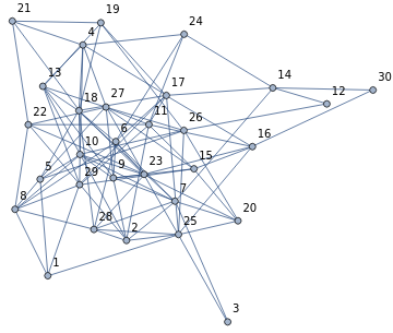
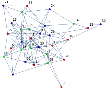
The following list of edges, E30, was created with the RandomGraph function and has 30 vertices and 100 edges.
In[]:=
E30={15,18,125,129,27,29,210,211,225,228,229,37,325,410,413,417,418,421,424,427,58,510,518,526,527,67,68,69,617,618,623,624,628,79,710,714,718,720,728,810,822,828,829,910,913,915,923,927,1013,1018,1023,1026,1029,1115,1116,1117,1122,1124,1127,1129,1214,1226,1318,1319,1327,1329,1417,1424,1430,1516,1520,1527,1529,1617,1623,1625,1630,1718,1719,1725,1729,1819,1821,1823,1828,1921,1926,2023,2025,2026,2122,2223,2227,2229,2325,2327,2328,2526,2528,2627}
Out[]=
{15,18,125,129,27,29,210,211,225,228,229,37,325,410,413,417,418,421,424,427,58,510,518,526,527,67,68,69,617,618,623,624,628,79,710,714,718,720,728,810,822,828,829,910,913,915,923,927,1013,1018,1023,1026,1029,1115,1116,1117,1122,1124,1127,1129,1214,1226,1318,1319,1327,1329,1417,1424,1430,1516,1520,1527,1529,1617,1623,1625,1630,1718,1719,1725,1729,1819,1821,1823,1828,1921,1926,2023,2025,2026,2122,2223,2227,2229,2325,2327,2328,2526,2528,2627}
In[]:=
Length[E30]
Out[]=
100
In[]:=
g30=Graph[E30,VertexLabelsAutomatic]
Out[]=
In[]:=
neighbors[G_,v_]:=DeleteCases[VertexList@NeighborhoodGraph[G,v],v]
For example, here are the neighbors of vertex 3
In[]:=
neighbors[E30,3]
Out[]=
{25,7}
We draw the graph.
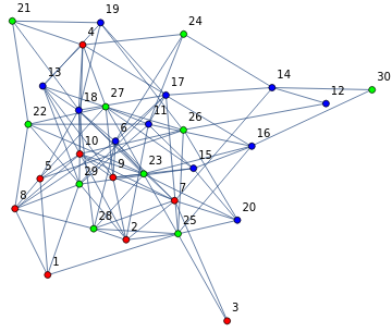
We arbitrarily color the first 10 vertices red, the next 10, blue, and the last 10, green.
In[]:=
reds=Range[10];blues=Range[11,20];greens=Range[21,30];
In[]:=
graph[r_,b_,g_][G_]:=Graph[G,VertexLabelsAutomatic,VertexStyleFlatten@{#Red&/@r,#Blue&/@b,#Green&/@g}]
Here is the image of the graph, colored as indicated.
In[]:=
What is the color of vertex 6? red. What constitutes “red”? For us “red” is the set of all vertices “colored red”, that is the set, reds. Same for other colors. So a “coloring” is just a partition of the vertices of the graph.
In[]:=
MemberQ[reds,6]
Out[]=
True
In[]:=
MemberQ[blues,6]
Out[]=
False
Thus vertex 6 is colored “red” but not “blue.”
To change the color of a vertex means to move it from one set to another. If it is in set “x” and we want to move it to set “y”, we need to delete it from set x, using DeleteCases and then add it to set y using Append. Say, we want to change the color of vertex 6 from red to blue.
In[]:=
reds=DeleteCases[reds,6]
Out[]=
{1,2,3,4,5,7,8,9,10}
In[]:=
blues=Append[blues,6]
Out[]=
{11,12,13,14,15,16,17,18,19,20,6}
Now vertex 6 is blue and not red.
We redraw the graph with this change.
In[]:=
graph[reds,blues,greens][E30]
Out[]=
We restore the original coloring.
In[]:=
reds=Range[10];blues=Range[11,20];greens=Range[21,30];
An edge is called mixed in the colored graph if its end vertices have different colors.
In[]:=
MixedEdgeQ[r_,b_,g_][UndirectedEdge[x_,y_]]:=Or[(MemberQ[r,x]&&!MemberQ[r,y]),(MemberQ[b,x]&&!MemberQ[b,y]),(MemberQ[g,x]&&!MemberQ[g,y])]
Next selects those edges whose vertices have different colors.
MixedEdges
In[]:=
MixedEdges[r_,b_,g_][E_]:=Select[E,MixedEdgeQ[r,b,g]]
In[]:=
MixedEdges[reds,blues,greens][E30]
Out[]=
{125,129,211,225,228,229,325,413,417,418,421,424,427,518,526,527,617,618,623,624,628,714,718,720,728,822,828,829,913,915,923,927,1013,1018,1023,1026,1029,1122,1124,1127,1129,1226,1327,1329,1424,1430,1527,1529,1623,1625,1630,1725,1729,1821,1823,1828,1921,1926,2023,2025,2026}
The mixing number of a vertex colored finite graph is the number of edges with different colored endpoints. Certainly this number is bounded by the number of edges of the graph.
In[]:=
MixingNumber[r_,b_,g_][E_]:=Length[MixedEdges[r,b,g][E]]
In[]:=
MixingNumber[reds,blues,greens][E30]
Out[]=
61
We need to get the set of neighbors of a vertex in a graph , that is, those vertices that share an edge with . Since the built-in Mathematica function includes the vertex itself, we remove it.
v
G
v
NeighborhoodGraph[G,v]
v
In[]:=
neighbors[G_,v_]:=DeleteCases[VertexList@NeighborhoodGraph[G,v],v]
For example, here are the neighbors of vertex 3 in E30
In[]:=
neighbors[E30,3]
Out[]=
{25,7}
Call a vertex a secure vertex in a 3-colored graph if has the same color as more than 1/3 of its neighbors in . If v is secure; there must be some color such that at most 1/3 of its neighbors have that color. If we switch the color of v to that color, it will increase the mixing number. Since the mixing number is bounded by the number of edges, we can’t do this indefinitely. (This is the idea behind the proof that an insecure coloring always exists.). If v is not secure, we call v insecure.
v
G
v
G
For example we show that vertex 13 which is blue, is insecure.
In[]:=
MemberQ[blues,13]
Out[]=
True
In[]:=
neighbors[E30,13]
Out[]=
{29,9,10,4,18,27,19}
In[]:=
neighbors[E30,13]⋂blues
Out[]=
{18,19}
So 13 is “blue” and has 2 blue neighbors and 2/7 < 1/3; thus vertex 13 is insecure. Also, vertex 20 is insecure as we show next.
In[]:=
MemberQ[blues,20]
Out[]=
True
In[]:=
neighbors[E30,20]
Out[]=
{25,7,26,23,15}
In[]:=
neighbors[E30,20]⋂blues
Out[]=
{15}
So vertex 20 has 5 neighbors, one of which are blue and 1/5 is less than 1/3. So vertex 20 is insecure.
Next we show that vertex 2 is secure.
In[]:=
MemberQ[reds,2]
Out[]=
True
In[]:=
neighbors[E30,2]
Out[]=
{25,29,7,9,10,11,28}
In[]:=
neighbors[E30,2]⋂reds
Out[]=
{7,9,10}
So vertex 2 which is red has 7 neighbors three of which are red and 3/7 > 1/3. So vertex 2 is secure.
In[]:=
The next function, color[ ] , labels the color of a vertex as either “red”, “blue”, or “green”, depending upon whether it is in reds, blues, or greens.
In[]:=
color[v_]:=Which[MemberQ[reds,v],"red",MemberQ[blues,v],"blue",MemberQ[greens,v],"green"]
In[]:=
color[13]
Out[]=
blue
In[]:=
color[20]
Out[]=
blue
In[]:=
color[2]
Out[]=
red
Next, we introduce SercureVertexQ, which tests for secure vertices.
In[]:=
SecureVertexQ[r_,b_,g_][G_,v_]:=Or[MemberQ[r,v]&&Length[neighbors[G,v]⋂r]>(1/3)Length[neighbors[G,v]],MemberQ[b,v]&&Length[neighbors[G,v]⋂b]>(1/3)Length[neighbors[G,v]],MemberQ[g,v]&&Length[neighbors[G,v]⋂g]>(1/3)Length[neighbors[G,v]]]
In[]:=
SecureVertexQ[reds,blues,greens][E30,20]
Out[]=
False
In[]:=
SecureVertexQ[reds,blues,greens][E30,13]
Out[]=
False
In[]:=
SecureVertexQ[reds,blues,greens][E30,2]
Out[]=
True
These are the secure vertices of E30.
In[]:=
sv=Select[Range[30],SecureVertexQ[reds,blues,greens][E30,#]&]
Out[]=
{1,2,3,5,6,7,8,9,10,11,12,14,15,16,17,19,22,23}
In[]:=
EdgeList[E30]
Out[]=
{15,18,125,129,27,29,210,211,225,228,229,37,325,410,413,417,418,421,424,427,58,510,518,526,527,67,68,69,617,618,623,624,628,79,710,714,718,720,728,810,822,828,829,910,913,915,923,927,1013,1018,1023,1026,1029,1115,1116,1117,1122,1124,1127,1129,1214,1226,1318,1319,1327,1329,1417,1424,1430,1516,1520,1527,1529,1617,1623,1625,1630,1718,1719,1725,1729,1819,1821,1823,1828,1921,1926,2023,2025,2026,2122,2223,2227,2229,2325,2327,2328,2526,2528,2627}
We define the corresponding function, , for any finite graph, G.
SecureVertices
In[]:=
SecureVertices[r_,b_,g_][G_]:=Select[VertexList[G],SecureVertexQ[r,b,g][G,#]&]
In[]:=
SecureVertices[reds,blues,greens][E30]
Out[]=
{1,5,8,2,7,9,10,11,3,17,6,23,14,22,15,16,12,19}
We use Union[ ] to order this list.
In[]:=
Union[{1,5,8,2,7,9,10,11,3,17,6,23,14,22,15,16,12,19}]
Out[]=
{1,2,3,5,6,7,8,9,10,11,12,14,15,16,17,19,22,23}
In[]:=
Union[{1,5,8,2,7,9,10,11,3,17,6,23,14,22,15,16,12,19}]sv
Out[]=
True
Next we restore the original coloring.
In[]:=
reds=Range[10];blues=Range[11,20];greens=Range[21,30];
We select the first element in the list of secure vertices .
v
sv
In[]:=
v=First@sv
Out[]=
1
In[]:=
color[1]
Out[]=
red
Thus vertex 1 is red and secure.
In[]:=
n[i_]:=neighbors[E30,i]
In[]:=
n[1]
Out[]=
{5,8,25,29}
The neighbors of vertex 1 are: {5,8,25,29}. We need to find their “colors” ;that is, what sets of the color partition they belong to. The function t[ i ] defined below which maps the color function “color” onto the set of neighbors of vertex i will do this for us.
In[]:=
t[i_]:=color[#]&/@n[i]
In[]:=
t[1]
Out[]=
{red,red,green,green}
In[]:=
In[]:=
Tally[t[1]]
Out[]=
{{red,2},{green,2}}
Note that “blue” is missing from the neighbors of vertex 1. To capture this in general we introduce the function Miss[ ].
In[]:=
Miss[v_]:=Complement[{"red","blue","green"},t[v]]
In[]:=
Miss[1]
Out[]=
{blue}
In[]:=
First[Miss[1]]
Out[]=
blue
In[]:=
t[5]
Out[]=
{red,red,red,blue,green,green}
Tally[ ] will tell us how many times each color occurs.
In[]:=
Tally[t[5]]
Out[]=
{{red,3},{blue,1},{green,2}}
In[]:=
t[13]
Out[]=
{green,red,red,red,blue,green,blue}
In[]:=
Tally[t[13]]
Out[]=
{{green,2},{red,3},{blue,2}}
In[]:=
color[13]
Out[]=
blue
We need a function that gives the color that occurs least often(maybe not at all!) in the neighborhood of a vertex. We introduce two functions SBTL and MinCol[ ] to do this.
In[]:=
SBTL[v_]:=SortBy[Tally[t[v]],Last][[1,1]]
In[]:=
SBTL[5]
Out[]=
blue
In[]:=
SBTL[13]
Out[]=
blue
The next function, MinCol[ ] selects the color that occurs least often in the neighborhood of a vertex v (if a color doesn’t occur at all, it selects that color).
In[]:=
MinCol[v_]:=If[Miss[v]≠{},First[Miss[v]],SBTL[v]]
In[]:=
Miss[13]
Out[]=
{}
In[]:=
MinCol[13]
Out[]=
blue
In[]:=
color[13]
Out[]=
blue
For example the color that occurs least often in vertex 1’s neighborhood is blue-- in fact it doesn’t occur at all.
In[]:=
color[1]
Out[]=
red
In[]:=
t[1]
Out[]=
{red,red,green,green}
In[]:=
MinCol[1]
Out[]=
blue
In[]:=
t[2]
Out[]=
{green,green,red,red,red,blue,green}
In[]:=
color[2]
Out[]=
red
In[]:=
MinCol[2]
Out[]=
blue
Now vertex 2 is red but is secure, since it has 3 red neighbor out of 7 neighbors and 3/7 > 1/3. If we changed its color to blue, it would increase its mixing number.
In[]:=
reds=Range[10];blues=Range[11,20];greens=Range[21,30];
The next function, ChangeColor[ ], looks at the neighborhood of a vertex v and selects the color that occurs least often(might even be missing!) and changes v’s color to that color. It is easy to see that this will increase the mixing number of the graph--if the vertex is secure!
In[]:=
ChangeColor[v_]:=Which[MemberQ[reds,v]&&MinCol[v]"blue",reds=DeleteCases[reds,v];blues=Append[blues,v];,MemberQ[reds,v]&&MinCol[v]"green",reds=DeleteCases[reds,v];greens=Append[greens,v];,MemberQ[blues,v]&&MinCol[v]"red",blues=DeleteCases[blues,v];reds=Append[reds,v];,MemberQ[blues,v]&&MinCol[v]"green",blues=DeleteCases[blues,v];greens=Append[greens,v];,MemberQ[greens,v]&&MinCol[v]"red",greens=DeleteCases[greens,v];reds=Append[reds,v];,MemberQ[greens,v]&&MinCol[v]"blue",greens=DeleteCases[greens,v];blues=Append[blues,v];]
In[]:=
ChangeColor[1]
Since vertex 1 was red and the minimum color in its neighborhood is blue, 1 has been deleted from reds and added to blues as the next computation shows. Thus, the color of vertex 1 has been changed from “red” to “blue.”
In[]:=
{reds,blues,greens}
Out[]=
{{2,3,4,5,6,7,8,9,10},{11,12,13,14,15,16,17,18,19,20,1},{21,22,23,24,25,26,27,28,29,30}}
Insecure 3-Colorings of a Graph
Insecure 3-Colorings of a Graph
In[]:=
reds=Range[10];blues=Range[11,20];greens=Range[21,30];
In[]:=
{reds,blues,greens}
Out[]=
{{1,2,3,4,5,6,7,8,9,10},{11,12,13,14,15,16,17,18,19,20},{21,22,23,24,25,26,27,28,29,30}}
The following short program produces an unfriendly coloring of any 3-colored graph.
In[]:=
InsecureColor[G_]:=Module[{v,sv},sv=SecureVertices[reds,blues,greens][G];While[sv≠{},v=First@sv;ChangeColor[v];sv=SecureVertices[reds,blues,greens][G];];{reds,blues,greens}]
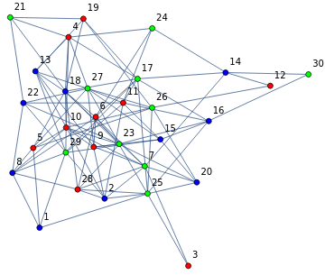
Here is an insecure 3-color partition of our graph starting with the original coloring.
In[]:=
InsecureColor[E30]
Out[]=
{{3,4,5,6,9,10,11,28,12,19},{13,14,15,16,18,20,1,8,2,22},{21,23,24,25,26,27,29,30,7,17}}
If we use this coloring, there will be no secure vertices.
In[]:=
reds={3,4,5,6,9,10,11,28,12,19};blues={13,14,15,16,18,20,1,8,2,22};greens={21,23,24,25,26,27,29,30,7,17};
In[]:=
SecureVertices[reds,blues,greens][E30]
Out[]=
{}
We display the “insecure” coloring of this graph.
In[]:=
Apply[graph,InsecureColor[E30]][E30]
Out[]=
We check that this is indeed “insecure “by showing each vertex is “insecure” given the current coloring.
In[]:=
Table[SecureVertexQ[reds,blues,greens][E30,i],{i,30}]
Out[]=
{False,False,False,False,False,False,False,False,False,False,False,False,False,False,False,False,False,False,False,False,False,False,False,False,False,False,False,False,False,False}
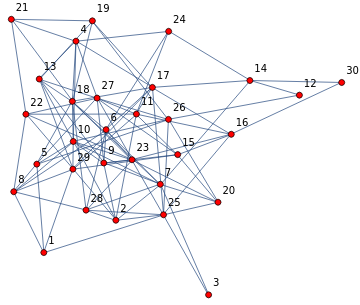
Suppose next we start with all red vertices. We can still apply our program to achieve an insecure coloring.
In[]:=
reds=Range[30];blues={};greens={};
In[]:=
graph[reds,blues,greens][E30]
Out[]=
In[]:=
Apply[graph,InsecureColor[E30]][E30]
Out[]=
In[]:=
Table[SecureVertexQ[reds,blues,greens][E30,i],{i,30}]
Out[]=
{False,False,False,False,False,False,False,False,False,False,False,False,False,False,False,False,False,False,False,False,False,False,False,False,False,False,False,False,False,False}
Defective Colorings
Defective Colorings
In the mid 1980s several authors “relaxed” the requirement of proper colorings that vertices that share an edge must be colored differently. One such “relaxation” was called in [ 1], “defective colorings.” According to [1], an (n,k)-coloring of a graph G is a n-coloring of its vertices such that for any vertex v, at most k of its neighbors have the same color as v. (An (n, 0)- coloring is the same as a proper k-coloring.) The following result is proved in a forthcoming paper[ 2 ].
Theorem 4. Let G be a finite graph with n vertices with maximal degree Δ(G). If 2 ⩽ k < n, then G is (k, ⌊Δ(G)/k⌋)-colorable where ⌊Δ(G)/k⌋ is the greatest integer less than or equal to Δ(G)/k. Moreover, this coloring can be found in polynomial time.
We show that an insecure coloring will produce (3, 3) coloring for our graph, g1, since the maximum degree of the graph is 11 (see below) and ⌊11/3⌋ = 3. Note that 3 is an upper bound; an insecure coloring might be a (3, u) - coloring for some u < 3.
In[]:=
Max[VertexDegree[E30]]
Out[]=
11
The following calculation shows that the above graph is in fact (3, 3) colorable. For each vertex i it counts the number of vertices in the neighborhood of i, that have i’s color. We see that this always less than or equal to 3!
In[]:=
Table[Length[Select[t[i],#color[i]&]],{i,30}]
Out[]=
{0,0,0,2,0,0,3,1,2,3,2,0,1,1,2,1,1,2,0,1,0,0,2,1,0,1,2,1,1,0}
Reference
[ 1 ] R. Cowen, L. Cowen and D. Woodall, “Defective colorings of graphs in surfaces: Partitions into subgraphs of bounded valency,” The Journal of Graph Theory, 10(2), 1986, 187 -195. https://doi.org/10.1002/jgt.3190100207.
[ 2 ] R. Cowen, Proportional Colorings of Graphs, to appear.
[ 1 ] R. Cowen, L. Cowen and D. Woodall, “Defective colorings of graphs in surfaces: Partitions into subgraphs of bounded valency,” The Journal of Graph Theory, 10(2), 1986, 187 -195. https://doi.org/10.1002/jgt.3190100207.
[ 2 ] R. Cowen, Proportional Colorings of Graphs, to appear.