ABSTRACT (original article): We investigate the transient and steady-state dynamics of the Bennati-Dragulescu-Yakovenko money game in the presence of probabilistic cheaters, who can misrepresent their financial status by claiming to have no money. We derive the steady-state wealth distribution per player analytically, and show how the presence of hidden cheaters can be inferred from the relative variance of wealth per player. In scenarios with a finite number of cheaters amidst an infinite pool of honest players, we identify a critical probability of cheating at which the total wealth owned by the cheaters experiences a second-order discontinuity. Below this point, the transition probability to lose money is larger than the probability to gain; conversely, above this point, the direction is reversed. We further establish a threshold cheating probability at which cheaters collectively possess half of the total wealth in the game. Lastly, we provide bounds on the rate at which both cheaters and honest players can gain or lose wealth, contributing to a deeper understanding of deception in asset exchange models. CITATION (original article): Kristian Blom, Dmitrii E. Makarov, Aljaž Godec (2025), Phys. Rev. Research 7, 013279. https://doi.org/10.1103/PhysRevResearch.7.013279
Load MaTex package and set color functions
Load MaTex package and set color functions
Monte-Carlo simulation for the money game with cheaters
Monte-Carlo simulation for the money game with cheaters
This is the core code which is used to generate trajectories of the money game with honest players and cheaters.
◼
The parameter “Nplayers” sets the total number of players in the game.
◼
The parameter “Ncheaters” sets the total number of cheaters in the game. The number of honest players is then given by “Nplayers-Ncheaters”.
◼
The parameter “Nsteps” sets the total number of discrete steps taken in the simulation.
◼
The parameter “Nmoney” sets the total amount of money in the game.
◼
The parameter “bias” introduces an additional bias in the exchange between two players, which is not studied in the manuscript “Hallmarks of Deception in Asset-Exchange Models”. For “bias > 1/2$” it is more likely that a richer player receives money from a poorer player. For “bias < 1/2$” it is more likely that a poorer player receives money from a richer player. In all sections below we set “bias=1/2”.
◼
The parameter “qc” sets the cheating probability of the cheaters.
◼
The parameter “trackall” determines whether all money is tracked or only the money of a single player. If “trackall = True” the money of all players will be tracked. If “trackall = False” the money of the first player will be tracked. And when “Ncheaters > 0” this player will be a cheater. When one needs to generate a very large trajectory it can be useful to set “trackall = False” to prevent memory issues.
moneygame[Nplayers_,Ncheaters_,Nsteps_,Nmoney_,bias_,qc_,trackall_]:=Module{playerlist=Range[Nplayers],values=ConstantArray[0,Nplayers]}, (*Setmoneytransactionvalues*) values[[1]]=1; values[[2]]=-1; (*Initializepath*) Clear[X,Y]; path=Array[X,Nsteps]; (*Setinitialconditionofmoneyperplayer;westartfromauniformdistributionofmoneyperplayer*) temp1=NmoneyNplayers; temp2=Floor[temp1]; temp3=ConstantArray[temp2,Nplayers]; temp3[[Nplayers]]=Nmoney-(Nplayers-1)temp2; If[trackall,X[1]=temp3,{X[1]=temp3[[1]],Y=temp3}]; (*Generaterandomwalkformoneygamewithcheaters*) Fori=2,i<=Nsteps,i++,(*Selecttworandomplayerswhichwillinterchangemoney*) players=RandomSample[playerlist], (*Createtransactionlist*) dm=Permute[values,players]; (*Determineamountofmoneypossessedbythetwoplayers*) {N1,N2}=If[trackall,X[i-1][[players[[1;;2]]]],Y[[players[[1;;2]]]]], (*Arewedealingwithcheatingplayers?Ifso,drawarandomnumberforthecheatingmove*) If[players[[1]]<=Ncheaters,If[RandomReal[]≤qc,N1=0]], If[players[[2]]<=Ncheaters,If[RandomReal[]≤qc,N2=0]], (*Monte-Carlomove*) IfN1==N2,If[N1!=0,If[trackall,X[i]=X[i-1]+dm,Y=Y+dm],If[trackall,X[i]=X[i-1],Y=Y]], If[N2>N1,dm*=-1], (*Thelinebelowcanbechangedtomakethegamesymmetricatm=0:If[RandomReal[]<=bias,X[i]=X[i-1]-dm,X[i]=X[i-1]]*) IfN1==0||N2==0,If[trackall,X[i]=X[i-1]-dm,Y=Y-dm], unfair=RandomReal[]<=bias, If[unfair,If[trackall,X[i]=X[i-1]+dm,Y=Y+dm],If[trackall,X[i]=X[i-1]-dm,Y=Y-dm]],If[!trackall,X[i]=Y[[1]]]; (*Outputtrajectory*) path
Analytical expressions
Analytical expressions
Here we list the analytical expressions for the wealth distribution which are derived and shown in the manuscript “Hallmarks of Deception in Asset-Exchange Models”.
These expressions will be used in later sections to plot the wealth distribution per player, and the average money owned by the cheaters and honest players.
These expressions will be used in later sections to plot the wealth distribution per player, and the average money owned by the cheaters and honest players.
Analytical expressions for the auxiliary functions; see Eq . (12)
Delta0[m_,q_,phi_]:=1+2*m*q+(1/3)(2*m-phi*q)^2;Delta1[m_,q_,phi_]:=(2/27)*(2*m-phi*q)^3+(1/3)*(2*m-phi*q)(1+2*m*q)+phi*q;
Steady - state probabilities at zero; see Eqs . (10) and (8), respectively
p0h[m_,q_,phi_]:=2*Sqrt[Delta0[m,q,phi]/3]Cos[(1/3)ArcCos[-(3/2)(Delta1[m,q,phi]/Delta0[m,q,phi])Sqrt[3/Delta0[m,q,phi]]]]+(phi*q-2m)/3;p0c[m_,q_,phi_]:=(p0h[m,q,phi]-q)/(1-q);
Steady - state probabilities; see Eqs . (11) and (9), respectively
pmh[k_,m_,q_,phi_]:=If[k>0,2*p0h[m,q,phi]*((1-p0h[m,q,phi])/(1+p0h[m,q,phi]))^k,p0h[m,q,phi]];pmc[k_,m_,q_,phi_]:=If[k>0,2*((p0h[m,q,phi]-q)/(1-q^2))*((1-p0h[m,q,phi])*(1+q)/((1+p0h[m,q,phi])*(1-q)))^k,p0c[m,q,phi]];
Steady - state probabilities in the large m limit; see Eqs . (16) and (17), respectively
p0hlim[m_,A_,phi_]:=(1+2A+Sqrt[1+4A(1+A-2phi)])/(4m)p0clim[m_,A_,phi_]:=(1-2A+Sqrt[1+4A(1+A-2phi)])/(4m)pmhlim[k_,m_,A_,phi_]:=If[k>0,2*p0hlim[m,A,phi]Exp[-2p0hlim[m,A,phi]*k],p0hlim[m,A,phi]]pmclim[k_,m_,A_,phi_]:=If[k>0,2*p0clim[m,A,phi]Exp[-2p0clim[m,A,phi]*k],p0clim[m,A,phi]]
Average money owned by a honest player or cheater; see Eqs . (26) and (25), respectively
mh[m_,q_,phi_]:=(1-p0h[m,q,phi])(1+p0h[m,q,phi])/(2p0h[m,q,phi]);mc[m_,q_,phi_]:=(1-p0h[m,q,phi])(1+p0h[m,q,phi])/(2(p0h[m,q,phi]-q));
Variance of total distribution
varm[m_,q_,phi_]:=m*++-m^2;
1
p0h[m,q,phi]
1-
2
p0h[m,q,phi]
p0h[m,q,phi]-q
-1+
2
p0h[m,q,phi]
p0h[m,q,phi]-phiq
Asymptotic solutions to Eq . (B13)
Collect[AsymptoticSolve[phi*(1-x)(1+x)/(2*x)+(1-phi)*(1-x)(1+x)/(2*(x-q))==m,x,{m,Infinity,2},Assumptions->{0<=phi<=1}],m]Collect[AsymptoticSolve[x^3+x^2(2*m-a*phi*m^(-B))-x(1+2*a*m^(1-B))+a*phi*m^(-B)==0/.{B->3/2},x,{m,Infinity,3},Assumptions->{0<=q<=1,0<=phi<=1,2/3<B<1}],m]FullSimplify[AsymptoticSolve[x^3+x^2(2*m-phi*q)-x(1+2*m*q)+phi*q==0,x,{m,Infinity,2},Assumptions->{0<=phi<=1,0<=q<=1}],Assumptions->{m>=0,0<=q<=1,0<=phi<=1}]
Out[]=
x+,xq++,x-2m-2-
phi
2m
-phi+
2
phi
4q
2
m
1-phi-+phi
2
q
2
q
2m
phi--2+2phi+2-3phi+
2
phi
2
q
2
q
4
q
4
q
2
phi
4
q
4q
2
m
q
2
phiq
2
Out[]=
x,x,x
Out[]=
x,x,x
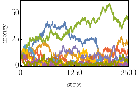
Plot money game simulation (used in Fig1. a-c)
Plot money game simulation (used in Fig1. a-c)
Set constants
Nplayers=10;Ncheaters=5;Nsteps=2500;Nmoney=100;bias=0.5;(*Thisparameterintroducesabiasintheexchangewhenitisnotequalto1/2*)qc=0.2;
Plot trajectories
ListPlotTranspose[moneygame[Nplayers,Ncheaters,Nsteps,Nmoney,bias,qc,True]],PlotRange->{{0,Nsteps},All}, Joined->True,Filling->False, PlotStyle->{{Thickness[0.009]},{Thickness[0.009]}}, FrameTrue,FrameStyleDirective[Thick,Black],FrameLabelMaTeX/@{steps,money}, FrameTicks->{{Table[{x,MaTeX[x,"DisplayStyle"->False,FontSize->24]},{x,Range[0,Nmoney,25]}],None},{Table[{x,MaTeX[x,"DisplayStyle"->False,FontSize->24]},{x,Range[0,Nsteps,Nsteps/2]}],None}}
Out[]=
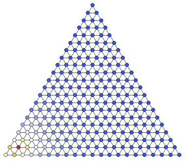
Animation of money game with 3 players
Animation of money game with 3 players
Set constants
Ncheaters=1;(*InthissectionNcheatersmustrangebetween0and3*)Nsteps=300;Nmoney=20;bias=0.5;qc=0.3;
Vertex translation; this names the vertices as a tuple (i, j, k)
vertextranslation=Flatten[Table[Table[(i-1)i/2+j->{i-j,j-1,Nmoney+1-i},{j,1,i}],{i,1,Nmoney+1}]];
Construct graph
graph=VertexReplace[ResourceFunction["TriangularGridGraph"][Nmoney],vertextranslation];
Animate random walk
ListAnimate[Table[{Graph[graph,VertexStyle->{v->Red},VertexSize->Large],graph=Graph[graph,VertexStyle->{v->Black},VertexSize->Large];},{v,moneygame[3,Ncheaters,Nsteps,Nmoney,bias,qc,True]}][[All,1]]]
A video of the output of the above animation:
Out[]=
Plot steady-state distribution of money game with 3 players (used in Fig. 1d-f)
Plot steady-state distribution of money game with 3 players (used in Fig. 1d-f)
Set constants
Ncheaters=1;(*InthissectionNcheatersmustrangebetween0and3*)Nsteps=200000;(*Makesurethisislargeenoughtosamplethesteady-state*)Nmoney=20;bias=0.5;qc=0.2;
Run trajectory
traj=moneygame[3,Ncheaters,Nsteps,Nmoney,bias,qc,True];
Vertex translation; this names the vertices as a tuple (i, j, k)
vertextranslation=Flatten[Table[Table[(i-1)i/2+j->{i-j,j-1,Nmoney+1-i},{j,1,i}],{i,1,Nmoney+1}]];
Construct graph + edge list + vertex list
graph=VertexReplace[ResourceFunction["TriangularGridGraph"][Nmoney],vertextranslation];elist=EdgeList[graph];vlist=VertexList[graph];
Construct table with steady - state probabilities
psstable=ParallelTable[Length[Position[traj,vlist[[i]]]]/Nsteps,{i,1,Length[vlist]}];
Find maximum occupancy probability to make color scheme more apparent
maxP=Max[psstable];
Optional : Partition trajectory into consecutive jumps to determine steady - state current
partitionedtraj=Partition[traj,2,1];
Optional : Construct table with steady - state fluxes
pfluxtable=ParallelTable[Length[Position[partitionedtraj,{elist[[i]][[1]],elist[[i]][[2]]}]]-Length[Position[partitionedtraj,{elist[[i]][[2]],elist[[i]][[1]]}]],{i,1,Length[elist]}];pfluxtable2=Round[pfluxtable/Nsteps,0.0007];
Optional : Show steady - state fluxes by adding arrows
graph2=graph;For[i=1,i<=Length[elist],i++,graph2=EdgeAdd[EdgeDelete[graph2,elist[[i]]],{If[pfluxtable2[[i]]==0,elist[[i]][[1]]elist[[i]][[2]],If[pfluxtable2[[i]]>0,elist[[i]][[1]]elist[[i]][[2]],elist[[i]][[2]]elist[[i]][[1]]]]}]]elist2=EdgeList[graph2];
Plot steady state distribution; if you want to also see fluxes change graph to graph2
Graph[graph,VertexStyleTable[vlist[[i]]{ColorData["TemperatureMap"][psstable[[i]]/maxP]},{i,1,Length[vlist]}],VertexSize->Large,EdgeStyle{Thick,Black}]
Out[]=
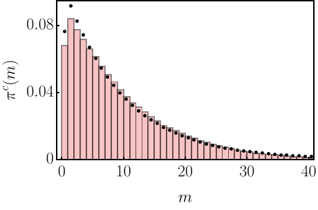
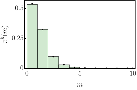
Plot steady state distribution of wealth (used for Fig. 3a-b)
Plot steady state distribution of wealth (used for Fig. 3a-b)
Set constants
Nplayers=20;Ncheaters=10;Nsteps=1000000;(*Makesurethisislargeenoughtosamplethesteady-state*)Nmoney=100;bias=0.5;qc=0.5;
Run trajectory
traj=moneygame[Nplayers,Ncheaters,Nsteps,Nmoney,bias,qc,True];
Plot histograms from numerical data
plt1=Histogram[{Flatten[Transpose[traj][[1;;Ncheaters]]]},{0,Nmoney,1},"Probability",PlotRange->{{0,40},{0,0.09}},FrameTrue,FrameStyleDirective[Thick,Black],Axes->False,PlotRangeClipping->True,FrameLabelMaTeX/@{"m","\\pi^{c}(m)"},ChartStyle->{{EdgeForm[{Black,Thickness[0.005]}]},{Col11}},FrameTicks->{{Table[{x,MaTeX[x,"DisplayStyle"->False,FontSize->20]},{x,{0,0.04,0.08}}],None},{Table[{x,MaTeX[x,"DisplayStyle"->False,FontSize->20]},{x,{0,10,20,30,40}}],None}}];plt2=Histogram[{Flatten[Transpose[traj][[Ncheaters+1;;]]]},{0,Nmoney,1},"Probability",PlotRange->{{0,10},{0,0.54}},ChartStyle->{{EdgeForm[{Black,Thickness[0.005]}]},{Col12}},FrameTrue,FrameStyleDirective[Thick,Black],PlotRangeClipping->True,FrameLabelMaTeX/@{"m","\\pi^{h}(m)"},FrameTicks->{{Table[{x,MaTeX[x,"DisplayStyle"->False,FontSize->20]},{x,{0,0.25,0.5}}],None},{Table[{x,MaTeX[x,"DisplayStyle"->False,FontSize->20]},{x,{0,5,10}}],None}}];
Plot analytical results given by Eq . (17)
plt3=ListPlot[Table[{k+1/2,pmc[k,Nmoney/Nplayers,qc,1-Ncheaters/Nplayers]},{k,0,40,1}],Filling->False,PlotStyle->{Thickness[0.008],Black,Dashed}];plt4=ListPlot[Table[{k+1/2,pmh[k,Nmoney/Nplayers,qc,1-Ncheaters/Nplayers]},{k,0,10,1}],Filling->False,PlotStyle->{Thickness[0.008],Black,Dashed}];
In[]:=
Show[plt1,plt3]
Out[]=
In[]:=
Show[plt2,plt4]
Out[]=
Plot steady state distribution of wealth in the large m limit (used for Fig. 3c)
Plot steady state distribution of wealth in the large m limit (used for Fig. 3c)
Set constants
Nplayers=20;Ncheaters=10;Nsteps=3000000;(*Makesurethisislargeenoughtosamplethesteady-state*)Nmoney=Nplayers*50;bias=0.5;qc=Nplayers/Nmoney;
Run trajectory
traj=moneygame[Nplayers,Ncheaters,Nsteps,Nmoney,bias,qc,True];
Plot histograms from numerical data
plt1=Histogram[{Flatten[Transpose[traj][[1;;Ncheaters]]]},{0,Nmoney,1},"Probability",ScalingFunctions->{"Log","Log"},FrameTrue,FrameStyleDirective[Thick,Black],Axes->False,PlotRangeClipping->True,ChartStyle->{{EdgeForm[None]},{Col11}}];plt2=Histogram[{Flatten[Transpose[traj][[Ncheaters+1;;]]]},{0,Nmoney,1},"Probability",PlotRange->{{1,400},{10^-4,0.06}},ChartStyle->{{EdgeForm[None]},{Col12}},ScalingFunctions->{"Log","Log"},FrameTrue,FrameStyleDirective[Thick,Black],PlotRangeClipping->True,FrameLabelMaTeX/@{"m",""},FrameTicks->{{Table[{x,MaTeX[x,"DisplayStyle"->False,FontSize->20]},{x,{10^-3,10^-2,10^-1}}],None},{Table[{x,MaTeX[x,"DisplayStyle"->False,FontSize->20]},{x,{10^0,10^1,10^2}}],None}}];
Plot analytical results given by Eq . (17)
plt3=ListLogLogPlot[Table[{k,pmclim[k,Nmoney/Nplayers,qc*Nmoney/Nplayers,1-Ncheaters/Nplayers]},{k,0,500,1}],Joined->True,PlotStyle->{Black,Thickness[0.01]},Filling->False];plt4=ListLogLogPlot[Table[{k,pmhlim[k,Nmoney/Nplayers,qc*Nmoney/Nplayers,1-Ncheaters/Nplayers]},{k,0,1000,1}],Joined->True,PlotStyle->{Black,Thickness[0.01]},Filling->False];
In[]:=
Show[plt2,plt4,plt1,plt3]
Out[]=
Plot average amount of money owned by the cheaters vs. the cheating probability qc (used in Fig. 4a-b)
Plot average amount of money owned by the cheaters vs. the cheating probability qc (used in Fig. 4a-b)
Set constants
Nplayers=300;Ncheaters=1;Nsteps=4000000;(*Makesurethisislargeenoughtosamplethesteady-statecorrectly*)Nmoney=500;bias=0.5;qc=Range[0,1,0.1];
Determine threshold and critical cheating probability; See Eqs . (28) and (13), respectively
qhalf=(1/2-Ncheaters/Nplayers)(Sqrt[(Nmoney/Nplayers)^2+4(1-Ncheaters/Nplayers)^2]-Nmoney/Nplayers)/((1-Ncheaters/Nplayers)^2);qcrit=Sqrt[(Nmoney/Nplayers)^2+1]-Nmoney/Nplayers;
Run trajectories; this part will take a while!
avgmoneycheaters=Table[{qc[[i]],(Ncheaters/Nmoney)Mean[moneygame[Nplayers,Ncheaters,Nsteps,Nmoney,bias,qc[[i]],False]]},{i,1,Length[qc],1}];avgmoneyfair=Table[{qc[[i]],1-Transpose[avgmoneycheaters][[2]][[i]]},{i,1,Length[qc],1}];
Plot average money
plt1=ListPlot[{avgmoneycheaters,avgmoneyfair},Frame->True,FrameStyleDirective[Thick,Black],FrameLabelMaTeX/@{"q_{c}"," "},PlotStyle->{{Black,PointSize[0.02]},{Black,PointSize[0.02]}},Joined->{False,False},Axes->False];plt2=Plot[{(Ncheaters/Nplayers)*mc[Nmoney/Nplayers,q,(Nplayers-Ncheaters)/Nplayers]/(Nmoney/Nplayers),((Nplayers-Ncheaters)/Nplayers)*mh[Nmoney/Nplayers,q,(Nplayers-Ncheaters)/Nplayers]/(Nmoney/Nplayers)},{q,0,1},PlotStyle->{{Col11,Thickness[0.012]},{Col12,Thickness[0.012]}},Frame->True,FrameStyleDirective[Thick,Black],FrameLabelMaTeX/@{"q_{c}",""},PlotRange->{{0,1},{0,1}},PlotStyle->{Thickness[0.01]},FrameTicks->{{Table[{x,MaTeX[x,"DisplayStyle"->False,FontSize->20]},{x,Range[0,1,0.2]}],None},{Table[{x,MaTeX[x,"DisplayStyle"->False,FontSize->20]},{x,Range[0,1,0.2]}],None}},Epilog->{{Directive[{Thickness[0.013],Col13,Dashed}],Line[{{qhalf,0},{qhalf,1}}]},{Directive[{Thickness[0.013],Black,Dashed}],Line[{{qcrit,0},{qcrit,1}}]}}];
In[]:=
Show[plt2,plt1]
Out[]=
Plot average amount of money owned by the cheaters upon decreasing the fraction of cheaters (Fig. 4c)
Plot average amount of money owned by the cheaters upon decreasing the fraction of cheaters (Fig. 4c)
Set constants
m=100/70;phi={0.85,0.9,0.95,0.975,0.995};
Set qcrit
qcrit=Sqrt[m^2+1]-m;
Plot average money owned by the cheaters; here we observe a second - order discontinuity
PlotEvaluate[Table[(1-phi[[i]])*mc[m,q,phi[[i]]]/m,{i,1,Length[phi]}]],Ifq>qcrit,1+,0,{q,0,1},PlotStyle->{{Col6,Thickness[0.01]},{Col7,Thickness[0.01]},{Col8,Thickness[0.01]},{Col9,Thickness[0.01]},{Col10,Thickness[0.01]},{Black,Thickness[0.01]}},PlotRange->{{0,1},{-0.05,1.05}},FrameTrue,FrameStyleDirective[Thick,Black],FrameLabelMaTeX/@{"q_{c}","\\langle M_c \\rangle/M"},FrameTicks->{{Table[{x,MaTeX[x,"DisplayStyle"->False,FontSize->20]},{x,Range[0,1,0.2]}],None},{Table[{x,MaTeX[x,"DisplayStyle"->False,FontSize->20]},{x,Range[0,1,0.2]}],None}},Epilog->{Directive[{Thickness[0.01],Black,Dashed}],Line[{{qcrit,0},{qcrit,1}}]}
-1+
2
q
2q*m
Out[]=

Plot speed limits for gaining and losing money vs. number of steps (Fig. 5a)
Plot speed limits for gaining and losing money vs. number of steps (Fig. 5a)
Set constants
Nplayers=100;Ncheaters=50;Nsteps=5000;Nmoney=10000;bias=0.5;qc={0,0.2,0.4,0.6,0.8};
Set number of independent simulations; the larger this is, the longer it takes
Nsims=200;
Initialize array containing amount of money owned by the cheaters per step
Mc=ConstantArray[0,{Length[qc],Nsteps}];
Run simulations for various values of the cheating probability, and collect the money owned by the cheaters
For[k=1,k<=Length[qc],k++,For[l=1,l<=Nsims,l++,Mc[[k,;;]]=Mc[[k,;;]]+Total[Transpose[moneygame[Nplayers,Ncheaters,Nsteps,Nmoney,bias,qc[[k]],True]][[1;;Ncheaters]]]]]
Normalize
Mc/=Nsims;
Compute upper bound given by Eq . 36 in the manuscript
Mcupper=Table[2*(Ncheaters/Nplayers)*(1-Ncheaters/Nplayers)*k,{k,0,Nsteps-1,1}];
Plot results
plt1A=ListPlot[Mcupper,Joined->True,PlotRange->{{0,Nsteps},All},PlotStyle->{{Black,Thickness[0.01]}},PlotRange->{{0,Nsteps},All},Frame->True,FrameStyleDirective[Thick,Black],Axes->False,FrameLabelMaTeX/@{"n","\\langle M_c(n) \\rangle-\\langle M_{c}(0) \\rangle "},FrameTicks->{{Table[{x,MaTeX[x,"DisplayStyle"->False,FontSize->20]},{x,Range[0,2500,1250]}],None},{Table[{x,MaTeX[x,"DisplayStyle"->False,FontSize->20]},{x,Range[0,5000,2500]}],None}}];plt2A=ListPlot[Table[Mc[[k,;;]]-Mc[[k,1]],{k,1,Length[qc]}],Joined->True,PlotStyle->{{Col1,Thickness[0.01]},{Col2,Thickness[0.01]},{Col3,Thickness[0.01]},{Col4,Thickness[0.01]},{Col5,Thickness[0.01]}}];
In[]:=
Show[plt1A,plt2A]
Out[]=
Plot speed limits for gaining and losing money vs. fraction of cheaters (Fig. 5b)
Plot speed limits for gaining and losing money vs. fraction of cheaters (Fig. 5b)
Set constants
Nplayers=100;Nsteps=500;Nmoney=10000;bias=0.5;qc={0,0.2,0.4,0.6,0.8};
Set number of independent simulations; the larger this is, the longer it takes
Nsims=10;
Initialize array containing amount of money owned by the cheaters per step and per fraction of cheaters
Mc2=ConstantArray[0,{Nplayers+1,Length[qc]}];
Compute average money for cheater
For[k=1,k<=Length[qc],k++,For[j=1,j<=Nplayers,j++,For[l=1,l<=Nsims,l++,{temp=Total[Transpose[moneygame[Nplayers,j,Nsteps,Nmoney,bias,qc[[k]],True]][[1;;j]]],Mc2[[j+1,k]]=Mc2[[j+1,k]]+(temp[[Nsteps]]-temp[[1]])/Nsteps}]]]
Normalize
Mc2/=Nsims;
Set theoretical bound
Mcupper2=Table[2*(i/Nplayers)*(1-i/Nplayers),{i,0,Nplayers}];
Plot result
plt1B=ListPlot[Mcupper2,Joined->True,PlotStyle->{{Black,Thickness[0.01]}},PlotRange->{{0,101},All},Frame->True,FrameStyleDirective[Thick,Black],Axes->False,FrameLabelMaTeX/@{"\\Phi_{c}","\\frac{\\langle M_c(n) \\rangle-\\langle M_{c}(0) \\rangle}{n} "},FrameTicks->{{Table[{x,MaTeX[x,"DisplayStyle"->False,FontSize->20]},{x,Range[0,0.5,0.25]}],None},{Table[{x,MaTeX[x,"DisplayStyle"->False,FontSize->20]},{x,Range[0,100,25]}],None}}];plt2B=ListPlot[Table[Mc2[[;;,j]],{j,1,Length[qc]}],Joined->True,PlotStyle->{{Col1,Thickness[0.01]},{Col2,Thickness[0.01]},{Col3,Thickness[0.01]},{Col4,Thickness[0.01]},{Col5,Thickness[0.01]}}];
In[]:=
Show[plt1B,plt2B]
Out[]=
CITE THIS NOTEBOOK
CITE THIS NOTEBOOK
Hallmarks of deception in asset-exchange models
by Kristian Blom, Dmitrii E. Makarov & Aljaž Godec
Wolfram Community, STAFF PICKS, March 11, 2025
https://community.wolfram.com/groups/-/m/t/3414673
by Kristian Blom, Dmitrii E. Makarov & Aljaž Godec
Wolfram Community, STAFF PICKS, March 11, 2025
https://community.wolfram.com/groups/-/m/t/3414673