ABSTRACT (original article): Recent astronomical observations obtained with the Kepler and TESS missions and their related ground-based follow-ups revealed an abundance of exoplanets with a size intermediate between Earth and Neptune (1 R⊕ ≤ R ≤ 4 R⊕). A low occurrence rate of planets has been identified at around twice the size of Earth (2 × R⊕), known as the exoplanet radius gap or radius valley. We explore the geometry of this gap in the mass–radius diagram, with the help of a Mathematica plotting tool developed with the capability of manipulating exoplanet data in multidimensional parameter space, and with the help of visualized water equations of state in the temperature–density (T–ρ) graph and the entropy–pressure (s–P) graph. We show that the radius valley can be explained by a compositional difference between smaller, predominantly rocky planets (<2 × R⊕) and larger planets (>2 × R⊕) that exhibit greater compositional diversity including cosmic ices (water, ammonia, methane, etc.) and gaseous envelopes. In particular, among the larger planets (>2 × R⊕), when viewed from the perspective of planet equilibrium temperature (Teq), the hot ones (Teq ≳ 900 K) are consistent with ice-dominated composition without significant gaseous envelopes, while the cold ones (Teq ≲ 900 K) have more diverse compositions, including various amounts of gaseous envelopes. CITATION (original article): Li Zeng et al (2021), New Perspectives on the Exoplanet Radius Gap from a Mathematica Tool and Visualized Water Equation of State, ApJ 923 247. https://doi.org/10.3847/1538-4357/ac3137
Introduction
Introduction
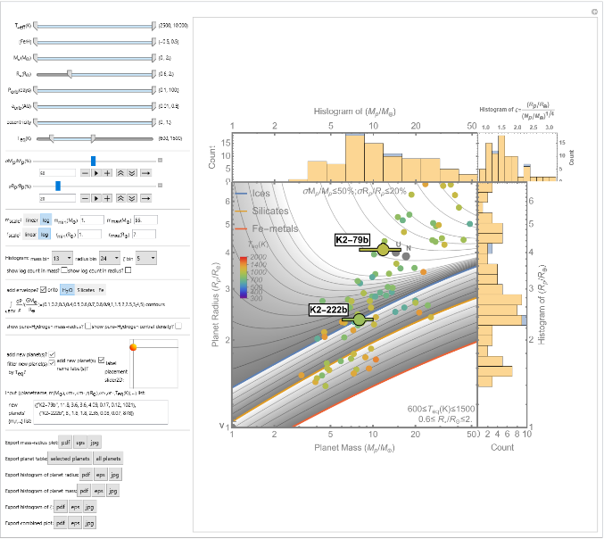
This is a Mathematica plotting tool developed to plot the exoplanet data in mass-radius diagram, and the relevant histograms (mass-histogram, radius-histogram, and \zeta-histogram). It is built on the functionality of Mathematica to Manipulate various input parameters when constructing the plots. For example, one important input parameter to separate exoplanet populations is the equilibrium temperature Teq , which is determined by the amount of host-stellar radiation that a planet receives per its unit surface area. By analogy, this is similar to the broad classification of any human disorder into either hot-nature or cold-nature according to the ancient Chinese, Ayurvedic, and Hellenistic medical knowledge. This manipulate function allows us to glean information from the observed planet population and make distinctions.
Another goal of this tool is to explore the possible origins of the exoplanet radius gap or radius valley, which corresponds to a low occurrence rate of observed planet population at around twice the size of Earth (2 × R⊕). We show that this radius gap or valley can be explained by a compositional difference between smaller, predominantly rocky planets (<2 × R⊕ ) and larger planets (>2 × R⊕ ) which exhibit greater compositional diversity including cosmic ices (water, ammonia, methane) plus gaseous envelopes. In particular, among the larger planets (>2 × R⊕ ), when viewed from the perspective of planet equilibrium temperature (Teq ), some hotter exoplanets (Teq>900 K) are consistent with ice-dominated composition without significant gaseous envelopes, while some colder exoplanets (Teq<900 K) seem to manifest various amounts of gaseous envelopes.
Another goal of this tool is to explore the possible origins of the exoplanet radius gap or radius valley, which corresponds to a low occurrence rate of observed planet population at around twice the size of Earth (2 × R⊕). We show that this radius gap or valley can be explained by a compositional difference between smaller, predominantly rocky planets (<2 × R⊕ ) and larger planets (>2 × R⊕ ) which exhibit greater compositional diversity including cosmic ices (water, ammonia, methane) plus gaseous envelopes. In particular, among the larger planets (>2 × R⊕ ), when viewed from the perspective of planet equilibrium temperature (Teq ), some hotter exoplanets (Teq>900 K) are consistent with ice-dominated composition without significant gaseous envelopes, while some colder exoplanets (Teq<900 K) seem to manifest various amounts of gaseous envelopes.
Importing data
Importing data
Import some mass-radius curves of isentropic pure-Hydrogen composition, calculated from the Hydrogen-EOS in Becker et al. ApJS 215,21 (2014). Mass-radius curves of the “isentropic” pure-Hydrogen compositions are added as an option here, particularly useful for the gas giant exoplanets such as those hot jupiters. “isentropic” here means that we assume the specific entropy within the gas envelope from its top to its bottom remains the same. This usually holds for deep fluidic envelopes due to internal convective motions caused by the presence of internal heat source from the central region of the planet. These “isentropic” pure-Hydrogen mass-radius curves counting from bottom upward in the mass-radius diagram are for specific entropy S (eV/1000K/atom)=0.3,0.4,0.5,0.6,0.7,0.8,0.9,and 1.0 correspondingly. One could see that both Saturn and Jupiter lie relatively close to the S (eV/1000K/atom)=0.3 curve, which is considered to be a relatively cold isentropic profile. The nominal surface of truncation of calculation for these mass-radius curves is taken to be at the density of 0.01 g/cc. Hydrogen EOS data are taken from Becker et al. ApJS 215,21 (2014) https://arxiv.org/abs/1411.4010
Set the working directory to notebook directory
In[]:=
SetDirectory[NotebookDirectory[]];
massradiusS03Becker=;
massradiusS04Becker=;
massradiusS05Becker=;
massradiusS06Becker=;
massradiusS07Becker=;
massradiusS08Becker=;
massradiusS09Becker=;
In[]:=
massradiusS10Becker=;
Interactive interface
Interactive interface
Wolfram Language notebook is attached at the end of the post.

Out[]=
CITE THIS NOTEBOOK
CITE THIS NOTEBOOK
Exoplanet mass-radius plotting and analyzing tool
by Li Zeng
Wolfram Community, STAFF PICKS, January 13, 2022
https://community.wolfram.com/groups/-/m/t/2445247
by Li Zeng
Wolfram Community, STAFF PICKS, January 13, 2022
https://community.wolfram.com/groups/-/m/t/2445247