This notebook explores the connection between quantum mechanics and number theory, particularly focusing on the reconstruction of one-dimensional potentials from given energy levels. The process, known as the inverse eigenvalue problem, utilizes the “dressing transformation” technique to generate potentials capable of reproducing predefined energy spectra. Examples include potentials derived from prime numbers, Fibonacci sequences, and sets of composite numbers, illustrating the versatility of the method in exploring connections between quantum systems and number-theoretical sequences.
The inverse eigenvalue problem in quantum mechanics deals with the reconstruction of a potential based on a given set of energy levels. This notebook demonstrates the use of the “dressing transformation” technique, a method rooted in soliton theory, to tackle this problem. We showcase this method’s application by generating potentials corresponding to various number sequences, such as prime numbers, Fibonacci numbers, and composite numbers. These examples highlight the fascinating intersection of quantum mechanics and number theory.
This article A. Ramani, B. Grammaticos, and E. Caurier, Phys. Rev. E 51, 6323 – Published 1 June 1995, http://dx.doi.org/10.1103/PhysRevE.51.6323 shows reconstruction of fractal potentials from energy levels.
Defining a function to reconstruct a potential from a given list of energy levels (evals). The potential is constructed over a specified range (xMax) and uses numerical methods (NDSolveValue) to iteratively determine the potential that best reproduces the given energy levels.
dressingTransformationPotentials[evals_,xMax_,opts___]:=Module[{ε,F,f,evals1=Sort[evals]-Max[evals],W=0&},Do[ε=evals1[[-k]];F=NDSolveValue[{f'[x]-f[x]^2+W[x]ε,f[0]0},f,{x,0,xMax},opts];W=Function@@{ξ,2ε+2F[ξ]^2-W[ξ]},{k,2,Length[evals1]}];Function@@{ξ,W[ξ]+Max[evals]}]
Generating a potential (V) whose energy levels correspond to the first 20 prime numbers. The potential is calculated over a range of 0 to 20.
V=dressingTransformationPotentials[Prime[Range[20]],20];
Visualize the generated potential (V).
Plot[V[Abs[x]],{x,-10,10}]
This code calculates the first 20 eigenvalues of the Schrödinger equation with the generated potential (V). The finite element method is used for numerical solution, and a maximum cell measure of 0.01 is specified for the mesh. This step verifies that the reconstructed potential indeed reproduces the desired energy levels (the first 20 prime numbers).
In[]:=
NDEigenvalues[-ψ''[x]+(V[Abs[x]])ψ[x],ψ,{x,-10,10},20,Method{"SpatialDiscretization"{"FiniteElement",{"MeshOptions"{"MaxCellMeasure"0.01}}}}]
Out[]=
{2.,3.,5.,7.,11.,13.,17.,19.,23.,29.,31.,37.,41.,43.,47.,53.,59.,61.,67.,71.}
Defining an alternative implementation of the dressingTransformationPotentials function. This implementation utilizes a different approach involving the solution of two coupled differential equations for functions ‘f’ and ‘g’ to construct the potential W.
dressingTransformationPotentials[evals_,xMax_,opts___]:=Module[{ε,f,g,evals1=Sort[evals]-Max[evals],W=0&},Do[ε=evals1[[-k]];W=NDSolveValue[{f'[x]-f[x]^2+W[x]ε,f[0]0,g'[x]==4f[x][x]-[x],g[0]==2ε-W[0]},{f,g},{x,0,xMax},opts][[2]],{k,2,Length[evals1]}];Function@@{ξ,W[ξ]+Max[evals]}]
′
f
′
W
Generating a potential (V) whose energy levels correspond to the first 20 prime numbers, similar to the previous implementation.
V=dressingTransformationPotentials[Prime[Range[20]],20]
Functionξ,71+
InterpolatingFunction

[ξ]Visualize the generated potential (V).
Plot[V[Abs[x]],{x,-10,10}]
The article Brandon P. van Zyl and David A. W. Hutchinson http://arxiv.org/abs/nlin/0304038 investigates the fractal nature of potentials reconstructed from the Riemann zeros and prime number sequences using two different inversion techniques. It concludes that both methods lead to the same fractal potential for a given set of energy levels, with a fractal dimension of 1.5 for the Riemann zeros and 1.8 for prime numbers.
Calculating the first 20 eigenvalues of the Schrödinger equation with the generated potential (V). This step verifies that the reconstructed potential indeed reproduces the desired energy levels (the first 20 prime numbers).
In[]:=
NDEigenvalues[-ψ''[x]+(V[Abs[x]])ψ[x],ψ,{x,-20,20},20,Method{"SpatialDiscretization"{"FiniteElement",{"MeshOptions"{"MaxCellMeasure"0.01}}}}]
Out[]=
{2.00001,3.00001,5.00003,7.00003,11.,13.0001,17.0001,19.0001,23.0001,29.0001,31.0001,37.0001,41.0002,43.0002,47.0001,53.0001,59.0002,61.0002,67.0001,71.0002}
Generating a list of the first 20 composite numbers within the range of 1 to 100, excluding the first 20 prime numbers.
compls=Take[Complement[Range[100],Prime[Range[20]]],20]
{1,4,6,8,9,10,12,14,15,16,18,20,21,22,24,25,26,27,28,30}
Generating a potential (V) corresponding to the list of composite numbers (compls). The potential is calculated over a range of 0 to 20.
V=dressingTransformationPotentials[compls,20];
Calculating the first 20 eigenvalues of the Schrödinger equation with the generated potential (V). This step confirms whether the reconstructed potential accurately reproduces the energy levels corresponding to the chosen composite numbers.
NDEigenvalues[-ψ''[x]+V[Abs[x]]ψ[x],ψ,{x,-12,12},20,Method{"SpatialDiscretization"{"FiniteElement",{"MeshOptions"{"MaxCellMeasure"0.02}}}}]
{1.,4.,6.,8.,9.,10.,12.,14.,15.,16.,18.,20.,21.,22.,24.,25.,26.,27.,28.,30.}
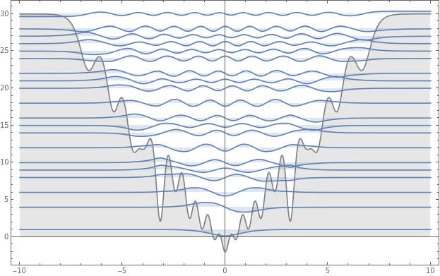
Calculating the eigenvalues and eigenfunctions for the Schrödinger equation with the generated potential (V) shifted upwards by 30 units.
ndse=NDEigensystem[-ψ''[x]+(V[Abs[x]]+30)ψ[x],ψ,{x,-10,10},20,Method{"SpatialDiscretization"{"FiniteElement",{"MeshOptions"{"MaxCellMeasure"0.02}}}}];
Visualizing both the generated potential (V) and the first 20 eigenfunctions of the Schrödinger equation, shifted downwards by 30 units to align with the potential. The plot highlights the relationship between the shape of the potential and the corresponding wavefunctions.
Show[{Plot[V[Abs[x]],{x,-10,10},PlotStyleGray,FillingAxis],Table[Plot[Evaluate[ndse[[2,j]][x]+ndse[[1,j]]-30],{x,-10,10},PlotRangeAll,FillingAxis,AxesOrigin{0,ndse[[1,j]]-30}],{j,20}]},FrameTrue]
Generate a potential (V) with energy levels based on the first 10 Fibonacci numbers (starting from the second Fibonacci number, 1).
V=dressingTransformationPotentials[Fibonacci[Range[2,12]],20];
Visualizing the generated potential (V).
Plot[V[Abs[x]],{x,-5,5},PlotRangeAll]
The first 10 eigenvalues of the Schrödinger equation with the generated potential (V). This step verifies whether the reconstructed potential accurately reproduces the energy levels corresponding to the first 10 Fibonacci numbers.
NDEigenvalues[-ψ''[x]+V[Abs[x]]ψ[x],ψ,{x,-15,15},10,Method{"SpatialDiscretization"{"FiniteElement",{"MeshOptions"{"MaxCellMeasure"0.005}}}}]
{1.,2.,3.,5.,8.,13.,21.,34.,55.,89.}
Related articles
Related articles
Cassettari, D., Marchukov, O. V., Carruthers, B., Kendell, H., Ruhl, J., Pierre, B. D. M., Zara, C., Weidner, C. A., Trombettoni, A., Olshanii, M., & Mussardo, G. (2024). Quantum dynamics of atoms in number-theory-inspired potentials (Version 1). arXiv. https://doi.org/10.48550/ARXIV.2410.13988
van Zyl, B. P., & Hutchinson, D. A. W. (2003). Riemann zeros, prime numbers, and fractal potentials. In Physical Review E (Vol. 67, Issue 6). American Physical Society (APS). https://doi.org/10.1103/physreve.67.066211
Ramani, A., Grammaticos, B., & Caurier, E. (1995). Fractal potentials from energy levels. In Physical Review E (Vol. 51, Issue 6, pp. 6323–6326). American Physical Society (APS). https://doi.org/10.1103/physreve.51.6323
CITE THIS NOTEBOOK
CITE THIS NOTEBOOK
Inverse eigenvalue problems: reconstructing fractal potentials from eigenvalue spectra
by Michael Trott
Wolfram Community, STAFF PICKS, October 23, 2024
https://community.wolfram.com/groups/-/m/t/3311726
by Michael Trott
Wolfram Community, STAFF PICKS, October 23, 2024
https://community.wolfram.com/groups/-/m/t/3311726