This is collaborative work by Philip Kuchel and Arthur Conigrave.
For several years a team led by AC has explored how intracellular calcium concentration responds to activation of the extracellular calcium-sensing receptor (CaSR), a class C G-protein coupled receptor (GPCR), in human cells. Using either transfected HEK-293 cells or native human parathyroid cells, living cells are loaded with the ratiometric dye Fura-2 AM, which is enzymatically converted inside the cell to the -sensitive fluorophore Fura-2.
[]
2+
Ca
i
2+
Ca
The imaging setup involves high-intensity UV excitation (340/380 nm) via a filter wheel [or fast-switching light emitting diodes (LEDs)], with emission captured at 510 nm using a high-sensitivity camera. Cells are maintained at physiological temperature (37 °C) and continuously perifused with physiological saline solutions.
At submaximal extracellular calcium levels (ₒ; 1.5-5.0 mM), oscillates rhythmically, with frequency increasing as ₒ rises. Beyond 5.0 mM, oscillations collapse into a sustained plateau. These dynamics are quantifiable using ionophores and calibrated /EGTA buffers.
[]
2+
Ca
[]
2+
Ca
i
[]
2+
Ca
[]
2+
Ca
i
2+
Ca
2+
Ca
A striking observation emerged: oscillation frequency is exquisitely temperature-sensitive. Even small shifts—down to 35 °C or up to 38 °C—significantly altered the frequency. This hinted at a possible thermosensory role for the CaSR.
To rigorously quantify these oscillations and their temperature dependence, we turned to wavelet analysis in Wolfram Language. Unlike Fourier methods, wavelets preserve time-localized features, making them ideal for analyzing non-stationary biological signals like oscillations.
[]
2+
Ca
i
Overview: A wavelet coefficient is the ‘score’ for how well a wavelet fits a component of the signal. High coefficients mean the wavelet closely matches the signal at that point — revealing important changes in oscillation frequency.
Provenance: As a PhD student (with PWK) David Szekely wrote the Mathematica script to perform the Morlet wavelet analysis, while PhD student (with AC) Sarah Brennan took this and ‘ran with it’ for analysing reams of beautiful oscillatory data like those shown here (see the original article for the details):
Related Articles
◼
Brennan, S. C., Mun, H. C., Delbridge, L., Kuchel, P. W., Conigrave, A. D. (2023) Temperature sensing by the calcium-sensing receptor, Front. Physiol. Memb. Physiol. & Memb. Biophys. 14, 2023, https://doi.org/10.3389/fphys.2023.1117352.
◼
Brennan, S. C., Mun, H.-C., Leach, K., Kuchel, P. W., Christopoulos, A., Conigrave, A. D. (2015) Impact of receptor density on calcium-sensing receptor mediated mobilization of intracellular . Endocrinol. 156, 1330-1342. https://doi.org/10.1210/en.2014-1771
2+
Ca
◼
Szekely, D., Brennan, S. C., Mun, H.-C., Conigrave, A. D., and Kuchel, P. W. (2009) Effectors of the frequency of calcium oscillations in HEK-293 cells: wavelet analysis and a computer model. Eur. Biophys. J. 39, 149-165. https://doi.org/10.1007/s00249-009-0469-2
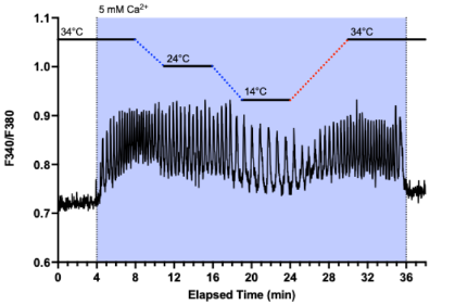
Figure 1. Temperature-dependent oscillations in fluorescence intensity recorded in human embryonic kidney cells (HEK-293). The dynamic signal (repetitive ~1 excitations at 340 and 380 nm; with emission centred on 510 nm) was captured using Fura-2, a -sensitive fluorescent probe, under high-resolution fluorescence microscopy equipped with digital image acquisition. The transfected cells had elevated expression of calcium-sensing receptors embedded in their plasma membranes.
-1
min
2+
Ca
More recently the script has been reworked to make use of the latest inbuilt commands in Wolfram Language. This is attached below. The script extracts oscillation frequencies with high temporal resolution, enables visualization of frequency shifts across temperature gradients, and compares signal structures across different [Ca²⁺]ₒ values.
Morlet wavelet analysis of simulated oscillatory data
Morlet wavelet analysis of simulated oscillatory data
Morlet wavelet analysis of synthetic fluorescence (microscope) intensities from HEK cells, indicative of oscillations in calcium concentration...PWK 251019
The annotation on graphs is minimalist to keep the syntax uncluttered...the context should be self-evident
Synthesize oscillatory fluorescence microscope data and plot them out
Synthesize oscillatory fluorescence microscope data and plot them out
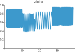
Choose four different arguments for the Sin functions used to generate the oscillatory data
In[]:=
f1=30;f2=10;f3=5;(*5/(2π)isthefrequencywithtimebeinginunitsofminutes...thisisequalto0.795oritsreciprocalistheperiodof1.25min...thiscanbeeasilyverifiedbymovingthecursorontheplotbelowandnotingthetimeintervalbetweenpeaks*)f4=20;synth=Table[{i,If[i<10,0.7+0.2Sin[f1i],If[i>10&&i<=17,0.6+0.2Sin[f2i],If[i>17&&i<=27,0.65+0.2Sin[f3i],0.75+0.2Sin[f4i]]]]},{i,1,39.07,0.0175}];(*Thesyntheticdata*)Length@%ListLinePlot[synth]
-1
min
Out[]=
2176
Out[]=
In[]:=
1/(2π/5.)
Out[]=
0.795775
Perform a Morlet continuous wavelet analysis on the data
Perform a Morlet continuous wavelet analysis on the data
The function automatically detects frequency regimes, but we choose our own scales then compute and display frequencies from which averages in various time domains can be calculated
In[]:=
dataClean=synth;(*thename"dataClean"isacarryoverfromwhenrealdatawere/areusedinthisscript*)time=dataClean[[All,1]];(*Sequenceoftimesusedintherecord*)signal=dataClean[[All,2]];(*Sequenceofsignalintensities*)dt=Mean[Differences[time]](*Valuethatiscalculatedfromrealfluorescencedata...withsyntheticdataitisadefinedvalue*)ScientificRound[x_]:=Floor[x+0.5](*TheparameterSampleRatemustbeanintegersotheexperimentalvaluemustberounded...weuseconventionalscientificroundingsoneedtospecifyourownfunctionasMathematicauses'bankingrounding'*)sampleRate=ScientificRound[1/dt]n=Length[signal];(*TheListlengthofthesignalisrequiredforiterationloopsbelow*)
Out[]=
0.0175
Out[]=
57
In[]:=
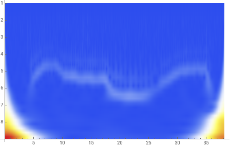
data=dataClean(*Thefluorescenceintensitydata...itiscleanherebutmaynotbewithrealdata*);intensityData=data[[All,2]];(*Theintensitydatafreeoftime*)nuOctaves=8;(*Thisdeteminesthefrequencyrangescannedbythewaveletanalysis*)nuVoices=4;(*Thisistheextentofsubdivisionoftheoctavesandagainisrelatedtotheresolutiononthefrequencyanalysis*)nuFreqs=nuOctaves*nuVoices;(*Totalnumberoffrequenciesofthewaveletsusedinprobingthedata*)(*ApplyContinuousWaveletTransformusingtheSampleRateasrounded1/dtfromabove*)cwd=ContinuousWaveletTransform[intensityData,MorletWavelet[],{nuOctaves,nuVoices},Padding->0.0,SampleRate->sampleRate](*Visualizethescalogram*)wsg=WaveletScalogram[cwd,ColorFunction->"TemperatureMap"]scales=cwd["Scales"](*Listofoctave-voicepairs*)wavs=cwd["Wavelet"](*SimplystatesthataMorletwaveletwasusedinthewaveletanalysis...othertypesareavailablethough*)
Out[]=
ContinuousWaveletData
Out[]=
Out[]=
{{1,1}1.02745,{1,2}1.22185,{1,3}1.45304,{1,4}1.72796,{2,1}2.0549,{2,2}2.44371,{2,3}2.90607,{2,4}3.45592,{3,1}4.10981,{3,2}4.88741,{3,3}5.81215,{3,4}6.91185,{4,1}8.21962,{4,2}9.77483,{4,3}11.6243,{4,4}13.8237,{5,1}16.4392,{5,2}19.5497,{5,3}23.2486,{5,4}27.6474,{6,1}32.8785,{6,2}39.0993,{6,3}46.4972,{6,4}55.2948,{7,1}65.7569,{7,2}78.1986,{7,3}92.9944,{7,4}110.59,{8,1}131.514,{8,2}156.397,{8,3}185.989,{8,4}221.179}
Out[]=
MorletWavelet[]
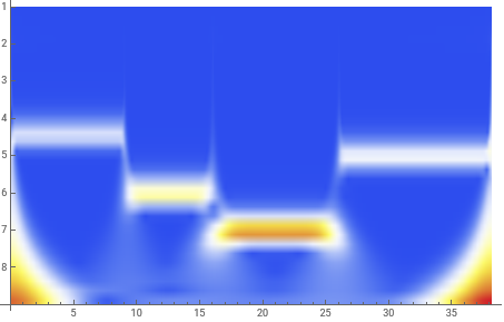
The scalogram clearly picks out the four data domains with their different frequencies.
We must now relate the ordinate on this scalogram to the various frequencies.
Normal[cwd] has all the data from the analysis so we can associate the “octave, voice” pairs (scales) with each corresponding frequency.
First inspect the output from Normal[cwd] and decide how to associate each scale pair with the respective coefficient (amplitudes) of the wavelets... there are nuOctaves x nuVoices such relationships.
In[]:=
Normal[cwd]
Out[]=
The IndexMap shows that the scales are divided into octaves (successive factors of 2) and voices (which are the subdivisions of the octaves)
In[]:=
cwd["IndexMap"]
Out[]=
{{1,1},{1,2},{1,3},{1,4},{2,1},{2,2},{2,3},{2,4},{3,1},{3,2},{3,3},{3,4},{4,1},{4,2},{4,3},{4,4},{5,1},{5,2},{5,3},{5,4},{6,1},{6,2},{6,3},{6,4},{7,1},{7,2},{7,3},{7,4},{8,1},{8,2},{8,3},{8,4}}
Convert the scales to frequencies using f = /(sampling time increment (dt) x scale) where is the central frequency of the Morlet wavelet...apparently it is 0.8125 and is internal to the Mathematica algorithm
f
c
f
c
In[]:=
factor=0.8125sampleRate;frequencyScale=Table[factor/scales[[i,2]],{i,1,nuFreqs}](*Herearethe32frequenciesusedinthisanalysis*)
Out[]=
{45.0751,37.9035,31.8729,26.8018,22.5375,18.9517,15.9365,13.4009,11.2688,9.47587,7.96823,6.70045,5.63439,4.73794,3.98411,3.35023,2.81719,2.36897,1.99206,1.67511,1.4086,1.18448,0.996028,0.837557,0.704298,0.592242,0.498014,0.418778,0.352149,0.296121,0.249007,0.209389}
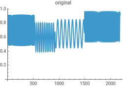
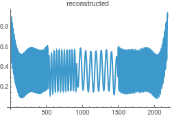
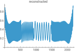
Reconstruct the data from the Morlet wavelet transform to check for consistency in the analysis...this uses the powerful InverseContinuousWaveletTransform
In[]:=
{ListLinePlot[intensityData,PlotLabel->"original"],ListLinePlot[InverseContinuousWaveletTransform[cwd],PlotLabel->"reconstructed"]}{ListLinePlot[dataClean,PlotLabel->"original"],ListLinePlot[InverseContinuousWaveletTransform[cwd],PlotLabel->"reconstructed"]}
Out[]=
,
Out[]=
,
Normal[cwd][[i, 2, k] contains the List of coefficients of the set of wavelets...all nuFreqs of them
The coefficients of the wavelet transform can be viewed as the z-axis values in a 3D matrix. We must associate each value with the time, k dt, which becomes the x-coordinate, and the scale which has been converted to frequency becomes the y-coordinate
In[]:=
dataNewAll=Table[{time[[k]],frequencyScale[[j]],Abs[Normal[cwd][[j,2,k]]]},{k,1,n},{j,1,nuFreqs}]dataNewTimeandCoeffs=Table[{time[[k]],Abs[Normal[cwd][[j,2,k]]]},{k,1,n},{j,1,nuFreqs}];
Out[]=
In[]:=
frequencyScale[[All]]
Out[]=
{45.0751,37.9035,31.8729,26.8018,22.5375,18.9517,15.9365,13.4009,11.2688,9.47587,7.96823,6.70045,5.63439,4.73794,3.98411,3.35023,2.81719,2.36897,1.99206,1.67511,1.4086,1.18448,0.996028,0.837557,0.704298,0.592242,0.498014,0.418778,0.352149,0.296121,0.249007,0.209389}
Now select a time point in the middle of each of the domains of different frequency and plot the coefficients of the wavelets on the y-axis versus the frequency on the x-axis...the position of the maximum then gives the central frequency of the respective data domain. Select time-points, 250, 750, 1250, and 1750...
In[]:=
procData1=Table[{(2π)frequencyScale[[k]],Transpose[dataNewTimeandCoeffs[[250]]][[2]][[k]]},{k,1,nuFreqs}];procData2=Table[{(2π)frequencyScale[[k]],Transpose[dataNewTimeandCoeffs[[750]]][[2]][[k]]},{k,1,nuFreqs}];procData3=Table[{(2π)frequencyScale[[k]],Transpose[dataNewTimeandCoeffs[[1250]]][[2]][[k]]},{k,1,nuFreqs}];procData4=Table[{(2π)frequencyScale[[k]],Transpose[dataNewTimeandCoeffs[[1750]]][[2]][[k]]},{k,1,nuFreqs}];
In[]:=
gph0=ListLinePlot[{procData1,procData2,procData3,procData4},PlotRange->{{0,40},{0,1.4}}]
Out[]=
Conclusion: From gph0 it is seen that each frequency used to generate the synthetic data has been returned in the wavelet analysis with maxima at 5, 10, 20 and 30 as required...I had to use a scaling factor of 2 π to get a consistent interpretation!
Check some more times...It can be seen that ‘edge effects’ creep in (at low values of frequency) but the maxima of the peaks are still in the correct positions
In[]:=
procData1=Table[{(2π)frequencyScale[[k]],Transpose[dataNewTimeandCoeffs[[100]]][[2]][[k]]},{k,1,nuFreqs}];procData2=Table[{(2π)frequencyScale[[k]],Transpose[dataNewTimeandCoeffs[[700]]][[2]][[k]]},{k,1,nuFreqs}];procData3=Table[{(2π)frequencyScale[[k]],Transpose[dataNewTimeandCoeffs[[1200]]][[2]][[k]]},{k,1,nuFreqs}];procData4=Table[{(2π)frequencyScale[[k]],Transpose[dataNewTimeandCoeffs[[2000]]][[2]][[k]]},{k,1,nuFreqs}];gph1=ListLinePlot[{procData1,procData2,procData3,procData4},PlotRange->{{0,40},{0,1.4}}]
Out[]=
Morlet wavelet analysis of real oscillatory data
Morlet wavelet analysis of real oscillatory data
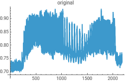
Morlet wavelet analysis of Sarah’s fluorescence (microscope) intensities from HEK cells, indicative of oscillations in calcium concentration...PWK 251018
The annotation on graphs is minimalist to keep the syntax uncluttered...the context should be self-evident
Real oscillatory fluorescence microscope data and plot it out
Real oscillatory fluorescence microscope data and plot it out
Set path to the uploaded Excel file
In[]:=
file="/Users/pkuc2216/Desktop/SarahRealData.xlsx";
Import entire workbook
In[]:=
dataAll=Import[file,"Data"];
Remove header etc
In[]:=
trimmedExcel=Partition[Drop[Flatten[dataAll],2],2];
Graph the data
In[]:=
gph1=ListLinePlot[trimmedExcel]
Out[]=
In[]:=
trimmedExcel;dataLength=Length[%]
Out[]=
2176
Perform a Morlet continuous wavelet analysis on the data
Perform a Morlet continuous wavelet analysis on the data
The function automatically detects frequency regimes, but we choose our own scales then compute and display frequencies from which averages in various time domains can be calculated
In[]:=
dataClean=trimmedExcel;time=dataClean[[All,1]];signal=dataClean[[All,2]];dt=Mean[Differences[time]]ScientificRound[x_]:=Floor[x+0.5]sampleRate=ScientificRound[1/dt]n=Length[signal];
Out[]=
0.0174525
Out[]=
57
The fluorescence intensity data
In[]:=
data=dataClean;(*ApplyContinuousWaveletTransformusingaMorletwavelet*)(*Assuming'data'isthetime-seriesfluorescenceintensity*)intensityData=data[[All,2]];nuOctaves=8;nuVoices=4;nuFreqs=nuOctaves*nuVoices;
Apply ContinuousWaveletTransform using the SampleRate as rounded 1/dt from above
In[]:=
cwd=ContinuousWaveletTransform[intensityData,MorletWavelet[],{nuOctaves,nuVoices},Padding->0.0,SampleRate->sampleRate]
Out[]=
ContinuousWaveletData
Visualize the scalogram
In[]:=
wsg=WaveletScalogram[cwd,ColorFunction->"TemperatureMap"]
Out[]=
In[]:=
scales=cwd["Scales"]wavs=cwd["Wavelet"](*ThissimplysaysthatIhaveusedaMorletwavelet*)
Out[]=
{{1,1}1.02745,{1,2}1.22185,{1,3}1.45304,{1,4}1.72796,{2,1}2.0549,{2,2}2.44371,{2,3}2.90607,{2,4}3.45592,{3,1}4.10981,{3,2}4.88741,{3,3}5.81215,{3,4}6.91185,{4,1}8.21962,{4,2}9.77483,{4,3}11.6243,{4,4}13.8237,{5,1}16.4392,{5,2}19.5497,{5,3}23.2486,{5,4}27.6474,{6,1}32.8785,{6,2}39.0993,{6,3}46.4972,{6,4}55.2948,{7,1}65.7569,{7,2}78.1986,{7,3}92.9944,{7,4}110.59,{8,1}131.514,{8,2}156.397,{8,3}185.989,{8,4}221.179}
Out[]=
MorletWavelet[]
The scalogram clearly picks out the four data domains with their different frequencies.
We must now relate the ordinate on this scalogram to the various frequencies.
Normal[cwd] has all the data from the analysis so we can associate the “octave, voice” pairs (scales) with each corresponding frequency.
First inspect the output from Normal[cwd] and decide how to associate each scale pair with the respective coefficient (amplitudes) of the wavelets... there are nuOctaves x nuVoices such relationships
In[]:=
Normal[cwd]
Out[]=
The IndexMap shows that the scales are divided into octaves (successive factors of 2) and voices (which are the subdivisions of the octaves)
In[]:=
cwd["IndexMap"]
Out[]=
{{1,1},{1,2},{1,3},{1,4},{2,1},{2,2},{2,3},{2,4},{3,1},{3,2},{3,3},{3,4},{4,1},{4,2},{4,3},{4,4},{5,1},{5,2},{5,3},{5,4},{6,1},{6,2},{6,3},{6,4},{7,1},{7,2},{7,3},{7,4},{8,1},{8,2},{8,3},{8,4}}
Convert the scales to frequencies using f = /(sampling time increment (dt) x scale) where is the central frequency of the Morlet wavelet...apparently it is 0.8125 and is internal to the algorithm
f
c
f
c
In[]:=
factor=0.8125sampleRate;frequencyScale=Table[factor/scales[[i,2]],{i,1,nuFreqs}]
Out[]=
{45.0751,37.9035,31.8729,26.8018,22.5375,18.9517,15.9365,13.4009,11.2688,9.47587,7.96823,6.70045,5.63439,4.73794,3.98411,3.35023,2.81719,2.36897,1.99206,1.67511,1.4086,1.18448,0.996028,0.837557,0.704298,0.592242,0.498014,0.418778,0.352149,0.296121,0.249007,0.209389}
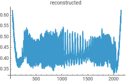
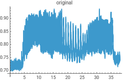
Reconstruct the data from the Morlet wavelet transform to check for consistency in the analysis...this uses the powerful InverseContinuousWaveletTransform
In[]:=
{ListLinePlot[intensityData,PlotLabel->"original"],ListLinePlot[InverseContinuousWaveletTransform[cwd],PlotLabel->"reconstructed"]}{ListLinePlot[dataClean,PlotLabel->"original"],ListLinePlot[InverseContinuousWaveletTransform[cwd],PlotLabel->"reconstructed"]}
Out[]=
,
Out[]=
,

Normal[cwd][[i, 2, k] contains the List of coefficients of the set of wavelets...all nuFreqs of them.
The coefficients of the wavelet transform can be viewed as the z-axis values in a 3D matrix. We must associate each value with the time, k dt, which becomes the x-coordinate, and the scale which has been converted to frequency becomes the y-coordinate
In[]:=
dataNewAll=Table[{time[[k]],frequencyScale[[j]],Abs[Normal[cwd][[j,2,k]]]},{k,1,dataLength},{j,1,nuFreqs}];dataNewTimeandCoeffs=Table[{time[[k]],Abs[Normal[cwd][[j,2,k]]]},{k,1,dataLength},{j,1,nuFreqs}]
Out[]=
In[]:=
frequencyScale[[All]]
Out[]=
{45.0751,37.9035,31.8729,26.8018,22.5375,18.9517,15.9365,13.4009,11.2688,9.47587,7.96823,6.70045,5.63439,4.73794,3.98411,3.35023,2.81719,2.36897,1.99206,1.67511,1.4086,1.18448,0.996028,0.837557,0.704298,0.592242,0.498014,0.418778,0.352149,0.296121,0.249007,0.209389}
Now select a time point in the middle of each of the domains of different frequency and plot the coefficients of the wavelets on the y-axis versus the frequency on the x-axis...the position of the maximum then gives the central frequency of the respective data domain. Select time-points, 250, 750, 1250, and 1750...
In[]:=
procData1=Table[{frequencyScale[[k]],Transpose[dataNewTimeandCoeffs[[250]]][[2]][[k]]},{k,1,nuFreqs}];procData2=Table[{frequencyScale[[k]],Transpose[dataNewTimeandCoeffs[[750]]][[2]][[k]]},{k,1,nuFreqs}];procData3=Table[{frequencyScale[[k]],Transpose[dataNewTimeandCoeffs[[1250]]][[2]][[k]]},{k,1,nuFreqs}];procData4=Table[{frequencyScale[[k]],Transpose[dataNewTimeandCoeffs[[1750]]][[2]][[k]]},{k,1,nuFreqs}];
In[]:=
gph0=ListLinePlot[{procData1,procData2,procData3,procData4},PlotRange->{{0,6},{0,0.6}}]
Out[]=
The code can be extended, for example, to automatically extract the mean and standard deviation of the frequency/period in a given time domain of the scalogram. These estimates of rate constants can then be graphed as a function of the known temperature of the cell sample at these times and thus estimate a temperature coefficient of the frequency.
CITE THIS NOTEBOOK
CITE THIS NOTEBOOK
Temperature sensing by the calcium-sensing receptor
by Philip Kuchel & Arthur Conigrave
Wolfram Community, STAFF PICKS, November 7, 2025
https://community.wolfram.com/groups/-/m/t/3572151
by Philip Kuchel & Arthur Conigrave
Wolfram Community, STAFF PICKS, November 7, 2025
https://community.wolfram.com/groups/-/m/t/3572151