Abstract: This notebook is aimed at showing the use of Mathematica in the study of nonlinear dynamics and in the construction of some typical tools, such as Poincaré maps and Fourier amplitude and phase spectra, which are useful for the classification of solutions. To clarify the concepts, a simple system is considered and some of its steady-state responses are shown.
Introduction
Introduction
Developments in the theory of dynamical systems since the early 1930s have been highly abstract in nature, and it was not until three decades later that physical models capable of concretely representing their behavior were described. Since then, numerous examples have been considered in physics, chemistry, mechanics and biology. Since most of the systems encountered were nonlinear, they could hardly be treated by classical closed-form methods of mathematical analysis. A great opportunity for the study of nonlinear dynamical systems has been provided by computers, which have made it possible to perform calculations with great precision and speed. Numerical simulations are, in fact, an important test bed for theory. The purpose of this notebook is to show how Mathematica, already at a fairly elementary level of use, can be adequately exploited by the end user, for both computation and visualization, in the study of the behavior of dynamical systems. Since little detail on nonlinear dynamics is given here, specific references must be considered. Indeed, there are many excellent books on this discipline and related topics. Among others, we mention the book by Thompson and Stewart [1] and that by Argyris et al. [2].
The governing equations
The governing equations
Let us consider a two-degree-of-freedom system that could represent a chain of two masses connected to each other and to a fixed ground with viscoelastic bonds. The interaction between each mass and the ground is linear with respect to both velocity and displacement. The mutual interaction between the masses is nonlinear with respect the displacement and linear with respect the velocity. In addition, one of the two masses is forced by a time-dependent term. The equations of motion, after a proper rescaling, would take the form:
..
x
1
b
10
x
1
b
12
x
1
x
2
x
1
c
12
x
1
x
2
3
(-)
x
1
x
2
..
x
2
b
12
x
1
x
2
b
23
x
2
c
12
x
1
x
2
c
23
x
2
3
(-)
x
1
x
2
(
1
) Usually, systems as this are addressed as non autonomous.
The space whose points uniquely represent all and only the possible states of Eq. (1) is called as the phase space, of dimension 2n, that is twice the number of degrees of freedom of the system. In phase space, evolution appears as a curve (or a sequence of points if the system is discrete).
Let us assume a certain solution of Eq. (1), for given initial conditions, is bounded for any t ≥ 0 and consider the stationary part, for : the trajectory cannot pass through all points of the phase space but is confined to moving in a compact (closed and bounded) manifold embedded in it.
To infer in a qualitative way the topology of the manifold on which the trajectory moves, let us consider the motion to be periodic and to be somehow modulated by another periodic motion, as the forcing term, for instance. The two motions can be represented as a trajectory given by their sum in the radial and transverse directions of a two-dimensional torus, an invariant subspace of phase space.
The ratio ρ between the modulated and modulating frequencies is called the rotation number. If ρ is a rational number, the motion is periodic with period ρT, where T is the period of the modulating motion, taken as fundamental. In such a case, the frequencies are commensurate and the trajectory is a closed curve on the torus, which is said a resonant torus. For this type of solution, it is possible to write explicitly, through a Fourier expansion, the amplitude spectrum consisting of equally spaced spikes. Typically, one calls the solutions with ρ=1 harmonic responses (with respect to the forcing term), and subharmonic responses those with ρ>1.
If ρ is irrational, the frequencies are incommensurate and the trajectory cannot close since the solution will not repeat periodically anymore. As the time increases, the trajectory becomes arbitrarily close to each point on the toroidal surface, densely filling it (for t→∞) in a neat way. In such a case the motion is quasiperiodic and the corresponding torus is said nonresonant.
Another class of possible solutions is that of chaotic responses. Chaotic motions are in fact long-term aperiodic behaviors that occur in a deterministic system, without any random or noisy input, as a consequence of nonlinearity. Differently from periodic and quasiperiodic behaviors, the chaotic responses exhibit a strongly sensitive dependence on initial conditions, making nearby trajectories diverge exponentially fast.
In the following, to illustrate these different behaviors, a number of solutions will be shown. They are taken from [3], where a large set of solutions of Eq. (1) was presented.
The space whose points uniquely represent all and only the possible states of Eq. (1) is called as the phase space, of dimension 2n, that is twice the number of degrees of freedom of the system. In phase space, evolution appears as a curve (or a sequence of points if the system is discrete).
Let us assume a certain solution of Eq. (1), for given initial conditions, is bounded for any t ≥ 0 and consider the stationary part, for
t≥
*
t
To infer in a qualitative way the topology of the manifold on which the trajectory moves, let us consider the motion
q
i
The ratio ρ between the modulated and modulating frequencies is called the rotation number. If ρ is a rational number, the motion is periodic with period ρT, where T is the period of the modulating motion, taken as fundamental. In such a case, the frequencies are commensurate and the trajectory is a closed curve on the torus, which is said a resonant torus. For this type of solution, it is possible to write explicitly, through a Fourier expansion, the amplitude spectrum consisting of equally spaced spikes. Typically, one calls the solutions with ρ=1 harmonic responses (with respect to the forcing term), and subharmonic responses those with ρ>1.
If ρ is irrational, the frequencies are incommensurate and the trajectory cannot close since the solution will not repeat periodically anymore. As the time increases, the trajectory becomes arbitrarily close to each point on the toroidal surface, densely filling it (for t→∞) in a neat way. In such a case the motion is quasiperiodic and the corresponding torus is said nonresonant.
Another class of possible solutions is that of chaotic responses. Chaotic motions are in fact long-term aperiodic behaviors that occur in a deterministic system, without any random or noisy input, as a consequence of nonlinearity. Differently from periodic and quasiperiodic behaviors, the chaotic responses exhibit a strongly sensitive dependence on initial conditions, making nearby trajectories diverge exponentially fast.
In the following, to illustrate these different behaviors, a number of solutions will be shown. They are taken from [3], where a large set of solutions of Eq. (1) was presented.
Numerical solutions
Numerical solutions
We rewrite Eq. (1) as a first order system:
equ=[t]x[3][t],[t]x[4][t],[t]PCos[tν]-x[1][t]-C12(x[1][t]-x[2][t])-μ-b10x[3][t]-b12(x[3][t]-x[4][t]),[t](C12(x[1][t]-x[2][t])+μ-C23x[2][t]+b12(x[3][t]-x[4][t])-b23x[4][t]);
′
x[1]
′
x[2]
′
x[3]
3
(x[1][t]-x[2][t])
′
x[4]
-1
γ
3
(x[1][t]-x[2][t])
The dimensions of the system and the vector of unknowns are equal to the dimension n of the phase space:
dimspace=4;unk=Table[x[i][t],{i,dimspace}];
Although not exploited here, any non autonomous system of dimension n may be treated as an autonomous system of larger dimension, simply by setting t as the variable and complementing the system with the equation = 1. The new system would therefore contain n+1 equations: its would be said a system of dimension n + 1/2 [4].
Some numerical solutions of the first order systems are computed for given sets of initial conditions and fixed parameters and several values of the circular frequency ν and the amplitude P of the forcing term:
x
n+1
x
n+1
Some numerical solutions of the first order systems are computed for given sets of initial conditions and fixed parameters and several values of the circular frequency ν and the amplitude P of the forcing term:
ICs=Table[x[i][0]5.0,{i,dimspace}];params={γ1.,μ1.,b100.05,b120.025,b230.025,C120.03,C230.08};forcepars={{0.73,0.2},{0.73,0.3},{0.73,1.5},{1.1,1.25},{1.2,0.9},{0.99,0.65},{1.07,0.5},{1.005,0.6},{0.86,0.25},{0.98,1.25},{1.11,0.5},{1.195,0.5}};
Integration spans a time interval long enough for the system to exit the transient phase, for a fixed number of cycles of the forcing:
tinit=0;Ncycles=5000;Tableperiod[i]=/.νforceparsi,1;tend[i]=Ncyclesperiod[i];,{i,Length[forcepars]};
2π
ν
We compute the numerical solutions (possibly in parallel, to save time):
maxsteps=;sys[i_]:=Join[equ/.params/.Inner[Rule,{ν,P},forcepars〚i〛,List],ICs];sol[i_,τ0_,τ1_,mx_]:=Flatten[NDSolve[sys[i],unk,{t,τ0,τ1},MaxStepsmx]];sols=If[$ProcessorCount>1,Parallelize[Table[sol[i,tinit,tend[i],maxsteps],{i,Length[forcepars]}]],Table[sol[i,tinit,tend[i],maxsteps],{i,Length[forcepars]}]];Table[eval[i]=Evaluate[sols〚i〛],{i,Length[forcepars]}];
7
10
The Poincaré map
The Poincaré map
The qualitative description of the solutions of Eq. (1) can be rather complicated. It is possible to reduce the dynamics by constructing a discrete dynamical system of co-dimension 1 with respect to the original continuous system, in which the relevant properties of the orbits are preserved. Such a discrete description is named stroboscopic map, return map, first recurrence map or Poincaré map, after Henri Poincaré (1854-1912) and it can be intuitively constructed as follows.
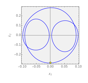
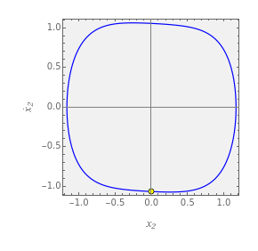
If we consider a flow lying on a two-dimensional torus, and set a specified plane, which we call a phase plane, transversely to the torus, the trajectory on the torus intersects the phase plane and, as time increases, the Poincaré map associates the first point to the second and so on, from which the name first recurrence map. The Poincaré section is normal to the flow in the sense that periodic orbits starting on that subspace flow through it and not parallel to it. The graph of the map is therefore built by collecting the intersection coordinates on the phase plane. We must observe that, in the general case, the Poincaré section is a hyper-surface of co-dimension 1, like the corresponding map. The resulting set of points from the Poincaré map forms a pattern that can be either regular or irregular.
If is a ρ-periodic function (with reference to the fundamental modulating motion) a set of ρ points will be mapped on the Poincaré section. In the case of quasiperiodic motion, the Poincaré map produces a closed curve in the phase plane, which can be interpreted, from a geometric point of view, as the cross-section of the torus. Finally, Poincaré maps exhibit a folded and stretched fractal structure in case of a chaotic response. The transition from a quasiperiodic motion to a chaotic one implies the breaking of the torus, which is indeed one of the strongest indicators of chaotic behavior.
Therefore, to classify the classification of solutions, we inspect the Poincaré plane. Here, we check how many points appear in the Poincaré plane after a given number of cycles.
If we consider a flow
x
i
If
x
i
Therefore, to classify the classification of solutions, we inspect the Poincaré plane. Here, we check how many points appear in the Poincaré plane after a given number of cycles.
prec=;inspectcycles=IntegerPartNcycles;Tablenumpoints[j,i]=LengthUnionNTableIntegerPart[prec{x[j][t]/.eval[i],x[j+2][t]/.eval[i]}],{t,tend[i]-inspectcyclesperiod[i],tend[i],period[i]},{i,Length[forcepars]},j,;
4
10
1
2
1
prec
dimspace
2
Fourier Analysis
Fourier Analysis
Here, we analyze the response of the system by means of the discrete Fourier transform [5], which converts a finite sequence of equally-spaced samples of a function into a sequence of complex values. Considering a time history, its Fourier representation gives values at positive and negative frequencies and a zero frequency value (often called as the DC component or DC offset, DC standing for direct current borrowed from electrical engineering and electronics), with the convention to put in the representation the DC component first, then the values at the positive frequencies, and finally those at the negative ones. To fix the ideas, let as choose a positive integer K and N = 2 K - 1 samples. The transform is organized as:
Text[Grid[{{Item["DC=X(1)",BackgroundLightBlue],"X(2)","...","X(K)",Item["X(K+1)",BackgroundLightOrange],Item["...",BackgroundLightOrange],Item["X(N)",BackgroundLightOrange]}},FrameAll,AlignmentCenter,ItemSizeAll]]
DC=X(1) | X(2) | ... | X(K) | X(K+1) | ... | X(N) |
where , 1 ≤ n ≤ N, is defined as
X(n)
X(n)x(r).
N
∑
r=1
-
2π(r-1)(n-1)
N
(
2
)Since , 2 ≤ κ ≤ K, where (·)stands for the complex conjugate of , information stored in entries associated with negative frequencies is redundant. Furthermore, it should be stressed that the values in Fourier transform can be scaled in a number of ways. The transform shown in Eq. (2) is that typically used in the field of digital signal processing.
For constructing the transform, we examine the last part of the system response, looking for a suitable time interval T (not necessarily equal to the period of the forcing) at whose endpoints and zero values occur. Indeed, such a choice may help in leakage suppression, without using specific windowing techniques. We locate the upper bound of the interval, first and then =-T. To save time in further computations, for responses with periodicity (with respect the forcing term) smaller or equal to a chosen “numax” we consider T be equal to one period of the response (which is equal to the period of the forcing if the periodicity of the response is 1). For the other case, the solutions are read on T equal to a suitably “reduced” number of cycles of the forcing.
X(κ)(-κ+N+2)
*
X
*
X
X(·)
X(n)
For constructing the transform, we examine the last part of the system response, looking for a suitable time interval T (not necessarily equal to the period of the forcing) at whose endpoints
t
0
t
1
t
1
t
0
t
1
Off[InterpolatingFunction::dmval];numax=10;reduced=200;Table(t1[j,i]=t/.FindRoot[(x[j][t]/.eval[i])0,{t,tend[i]-3/4period[i],tend[i]-period[i]/4},AccuracyGoalAutomatic];t0[j,i]=If[numpoints[j,i]≤numax,t1[j,i]-numpoints[j,i]period[i],t/.FindRoot[(x[j][t]/.eval[i])(x[j][t]/.eval[i]/.tt1[j,i]),{t,t1[j,i]-(reduced+2)period[i],t1[j,i]-(reduced-2)period[i]},AccuracyGoalAutomatic]];T[j,i]=t1[j,i]-t0[j,i];),{i,Length[forcepars]},j,;
dimspace
2
Once the proper T is defined, an odd number N of samples is chosen, to which corresponds a time step Δt. The function is then sampled:
k=4;Tablerounded[j,i]=Round;nsamples[j,i]=If[OddQ[rounded[j,i]],rounded[j,i],rounded[j,i]+1];Δt[j,i]=;sample[j,i]=Table[{t,x[j][t]/.eval[i]},{t,t0[j,i],t1[j,i]-Δt[j,i],Δt[j,i]}];,{i,Length[forcepars]},j,;
k
2
T[j,i]
period[i]
T[j,i]
nsamples[j,i]
dimspace
2
The sampling rate Δf = 1/Δt, that is the number of samples per time unit (one second, for instance) is crucial to fulfill the sampling theorem showing that a function can be properly sampled only if it does not contain frequency components above one-half of the sampling rate [6].
Now, we compute the Fourier transform, adopting the Fourier parameters of digital signal processing, in agreement with the definition given in Eq. (2):
Now, we compute the Fourier transform, adopting the Fourier parameters of digital signal processing, in agreement with the definition given in Eq. (2):
Tablefouriert[j,i]=Chop[Fourier[sample[j,i]〚All,2〛,FourierParameters{1,-1}]],{i,Length[forcepars]},j,;
dimspace
2
This also allows reconstructing the sampled function (which is now treated as periodic of period T) as a sum of sinusoids:
g(t)=sin(2πt+)
K
∑
n=1
A
n
f
n
Φ
n
(
3
)where
f
n
Δf
N
n-1
NΔt
n-1
T
(
4
)A
1
Abs()
X
1
N
A
n
2Abs()
X
n
N
(
5
)Φ
n
π
2
X
n
(
6
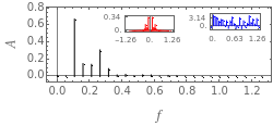
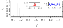
)All this information can be organized in single-sided and double-sided amplitude spectra and in phase spectrum.
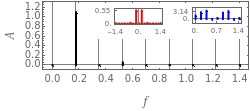
The fundamental frequency is found in correspondence of max(), 2 ≤ n ≤ K.
The fundamental frequency
0
f
n
A
n
Tablef[j,i]=Table,n,;A[j,i]=AbsJoin,Takefouriert[j,i],2,;Φ[j,i]=+Arg[fouriert[j,i]];greconstr[j,i]=A[j,i]hSin[2πf[j,i]〚h〛t+Φ[j,i]〚h〛];singlesidedspectrum[j,i]=Transpose[{f[j,i],A[j,i]}];fds[j,i]=Join[f[j,i],-Reverse[Drop[f[j,i],1]]];doublesidedspectrum[j,i]=Transposefds[j,i],;phasespectrum[j,i]=Transpose[{fds[j,i],Φ[j,i]}];maxamplitude[j,i]=Max[Drop[A[j,i],1]];f0[j,i]=Drop[singlesidedspectrum[j,i],1]Position[singlesidedspectrum[j,i],maxamplitude[j,i]]1,1,1;,{i,Length[forcepars]},j,;
n-1
T[j,i]
nsamples[j,i]+1
2
2
nsamples[j,i]
First[fouriert[j,i]]
2
nsamples[j,i]+1
2
π
2
nsamples[j,i]+1
2
∑
h=1
Abs[fouriert[j,i]]
nsamples[j,i]
dimspace
2
Toroidal coordinates
Toroidal coordinates
An interesting three-dimensional representation of a flow can be given, based on toroidal coordinates, defined as
xT[x__,ω_]:=+xCos[ωt];yT[x__,ω_]:=+xSin[ωt];zT[x__]:=x;
1
ω
1
ω
∂
t
Some delayed functions for graphics
Some delayed functions for graphics
For graphics, the responses framed in between and are translated back, in order the left and right endpoints of the time interval are set =0 and =T, respectively.
t
0
t
1
⋆
t
0
⋆
t
1
Table(ξ[j,i]=(x[j][t]/.eval[i]/.tt+t0[j,i]);ξ[j+2,i]=(x[j+2][t]/.eval[i]/.tt+t0[j,i]);),{i,Length[forcepars]},j,;
dimspace
2
A number of delayed functions to plot time histories (1), phase trajectories (2), Poincaré maps (3), amplitude and phase spectra (4), toroidal trajectories (5) and graphical tables of results (6) are defined in the following.
1. Time history
1. Time history
2. Phase trajectory
2. Phase trajectory
3. Poincaré map
3. Poincaré map
4. Amplitude and phase spectra
4. Amplitude and phase spectra
5. Toroidal trajectory
5. Toroidal trajectory
6. Graphical table of results
6. Graphical table of results
Results and graphics
Results and graphics
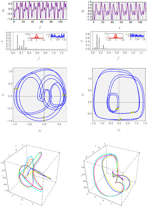
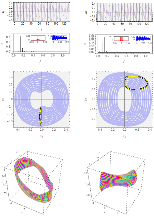
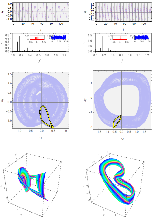
Some periodic and multi-periodic, quasiperiodic and chaotic solutions are reported in this section.
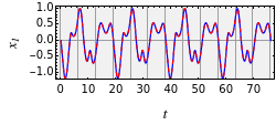
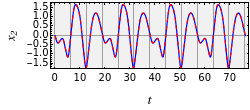
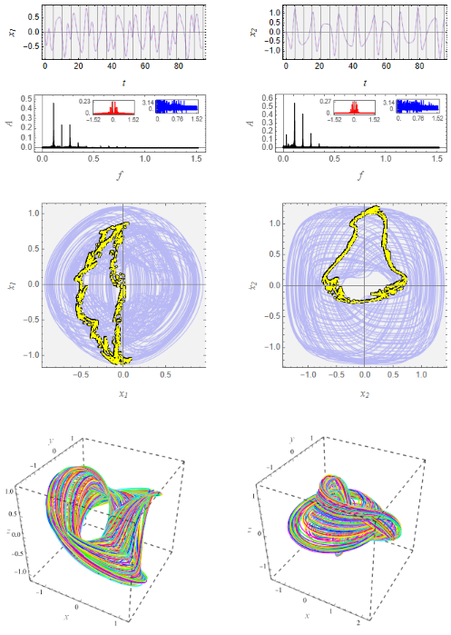
Graphics are organized in tables with two columns (for and , respectively) and four rows:
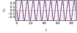
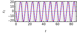
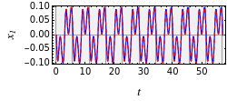
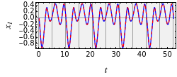
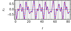
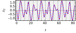
(i) the top panel reports time histories of “translated” (blue solid) and “reconstructed” (red dashed) responses. Vertical gray lines show the periodicity of the forcing term;
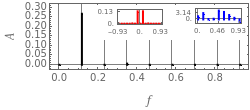
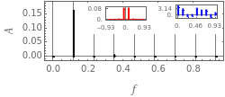
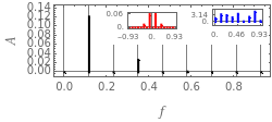
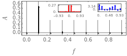
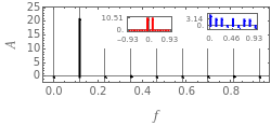
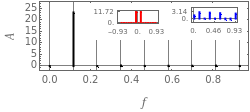
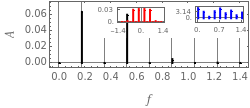
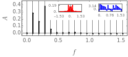
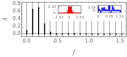
(ii) the second panel from top reports the single-sided amplitude spectrum and, in the two inset boxes, the double-sided spectrum (red colored) and the phase spectrum at positive frequencies (blue colored);
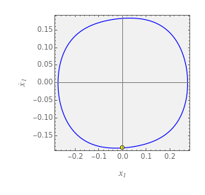
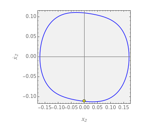
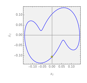
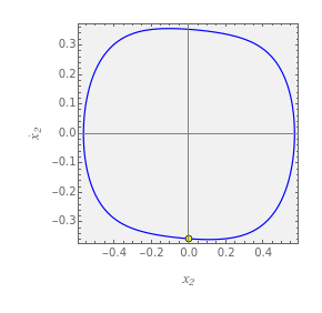
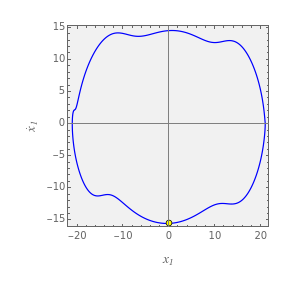
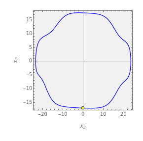
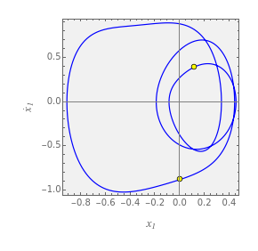
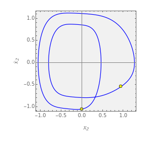
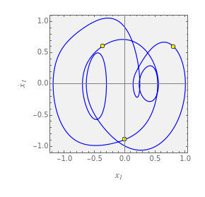
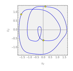
(iii) the third panel from top reports phase trajectories with superimposed Poincaré maps, as colored dots;
(iv) the lower panel shows the toroidal trajectory, displayed in a color hue corresponding to the time progression.
Graphics are organized in tables with two columns (for
x
1
x
2
(i) the top panel reports time histories of “translated” (blue solid) and “reconstructed” (red dashed) responses. Vertical gray lines show the periodicity of the forcing term;
(ii) the second panel from top reports the single-sided amplitude spectrum and, in the two inset boxes, the double-sided spectrum (red colored) and the phase spectrum at positive frequencies (blue colored);
(iii) the third panel from top reports phase trajectories with superimposed Poincaré maps, as colored dots;
(iv) the lower panel shows the toroidal trajectory, displayed in a color hue corresponding to the time progression.
Periodic solutions
Periodic solutions
Period 1
Period 1
k=1;graph[k,10,1,1,500,Thickness[0.006],Blue,0.025,Yellow,250]
 |  |


k=2;graph[k,10,1,1,500,Thickness[0.006],Blue,0.025,Yellow,250]
 |  |

k=3;graph[k,10,1,1,500,Thickness[0.006],Blue,0.025,Yellow,250]
 |  |

k=4;graph[k,10,1,1,500,Thickness[0.006],Blue,0.025,Yellow,250]
 |  |

Period 2
Period 2
k=5;graph[k,10,1,1,500,Thickness[0.006],Blue,0.025,Yellow,250]
 |  |

Period 3
Period 3
k=6;graph[k,12,1,1,500,Thickness[0.006],Blue,0.025,Yellow,250]
 |  |
Period 5
Period 5
k=7;graph[k,14,1,1,500,Thickness[0.006],Blue,0.022,Yellow,250]
 |  |
Period 6
Period 6
k=8;graph[k,18,1,1,500,Thickness[0.006],Blue,0.022,Yellow,250]
Quasiperiodic solutions
Quasiperiodic solutions
k=9;graph[k,18,0.8,1,500,Thin,Blue,0.01,Yellow,250]
k=10;graph[k,18,0.68,1,500,Thin,Blue,0.01,Yellow,250]
Chaotic solutions
Chaotic solutions
k=11;graph[k,18,1,1,500,Thin,Blue,0.01,Yellow,250]
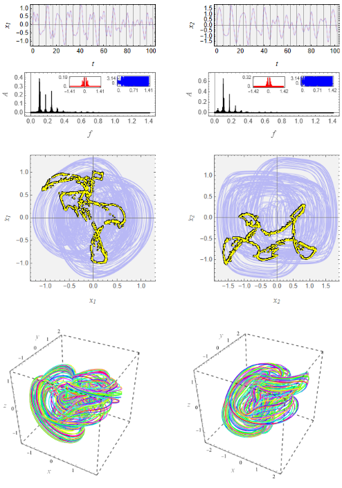
k=12;graph[k,18,0.8,1,500,Thin,Blue,0.01,Yellow,250]
Conclusions
Conclusions
With the aim of showing how Mathematica can be easily exploited in the analysis of nonlinear dynamical systems, two simultaneous ordinary differential equations are considered in this notebook. Some periodic, quasiperiodic and chaotic solutions are computed and visualized in terms of time histories and phase trajectories. Typical tools, as Poincaré maps, amplitude and phase spectra, are built using functions available in Mathematica.
References
References
[1] J. M. T. Thompson and H. B. Stewart, Nonlinear Dynamics and Chaos, 2nd ed., Wiley, Chichester, 2002
[2] J. H. Argyris, G. Faust, M. Haase, R. Friedrich, An Exploration of Dynamical Systems and Chaos - Completely Revised and Enlarged Second Edition. Springer Berlin, Heidelberg, 2015. https://doi.org/10.1007/978-3-662-46042-9
[3] E. Babilio. La Dinamica Nonlineare dei Sistemi a Due Gradi di Libertà (Italian for “Nonlinear Dynamics of Two-Degree-of-Freedom Systems”). Unpublished Master’s Thesis. In Italian. University of Naples “Federico II”, Naples, Italy, 1999.
[4] J. K. Hale, H. Koçak. Dynamics and Bifurcationss. Springer-Verlag New York, Inc., 1991. https://doi.org/10.1007/978-1-4612-4426-4
[5] J. S. Bendat, A. G. Piersol. Random Data: Analysis and Measurement Procedures. John Wiley & Sons, Inc., 2010. doi:10.1002/9781118032428
[6] S. W. Smith. The Scientist and Engineering’s Guide to Digital Signal Processing. California Technical Publishing, 1997.
CITE THIS NOTEBOOK
CITE THIS NOTEBOOK
Some basics on the responses of nonlinear dynamical systems
by Enrico Babilio
Wolfram Community, STAFF PICKS, September 15, 2023
https://community.wolfram.com/groups/-/m/t/3013411
by Enrico Babilio
Wolfram Community, STAFF PICKS, September 15, 2023
https://community.wolfram.com/groups/-/m/t/3013411