In[]:=
deploy
Uploading to newton/ill-conditioned.nb
Out[]=
Ill - conditioning example
Ill - conditioning example
Correlated coordinates
Correlated coordinates
In[]:=
ones=v2c@{1,1};A=ones.Transpose[ones]
Out[]=
{{1,1},{1,1}}
In[]:=
v2c[{1,1}].Transpose[v2c[{1,1}]]
Out[]=
{{1,1},{1,1}}
In[]:=
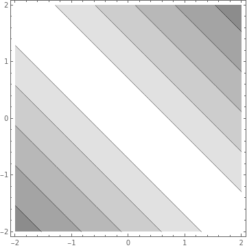
plt=ContourPlot[Sqrt[0.5{x1,x2}.A.{x1,x2}],{x1,-2,2},{x2,-2,2},ColorFunction->Function[GrayLevel[1-.45#]]]
Out[]=
In[]:=
f[{x1_,x2_}]:=0.5{x1,x2}.A.{x1,x2}
In[]:=
f[{1,0}]
Out[]=
0.5
In[]:=
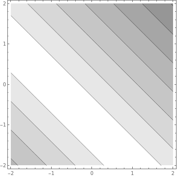
x0=v2c@{1,0};g0={1,1};h[{x1_,x2_}]:=(x=v2c@{x1,x2};f[{1,0}]+g0.x+.5x.A.x);ContourPlot[Sqrt[h[{x1,x2}]],{x1,-2,2},{x2,-2,2},ColorFunction->Function[GrayLevel[1-.45#]]]
Out[]=
In[]:=
f[{1,0}]h[{0,0}]
Out[]=
0.5{{0.5}}
In[]:=
LinearSolve[H,{1,1}]
Out[]=
{1,0}
In[]:=
{1,0}.H.PseudoInverse[H.H]
Out[]=
,
1
4
1
4
In[]:=
{1,0}.Inverse[H.H+lIdentityMatrix[2]].H
Out[]=
{0.249999,0.249999}
In[]:=
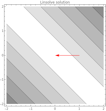
x0={1,0};sol1=LinearSolve[H,{1,1}];Show[plt,Graphics[{Red,Arrow[{{1,0},x0-sol1}]}],PlotLabel"Linsolve solution"]
Out[]=
In[]:=
sol1
Out[]=
{1,0}
In[]:=
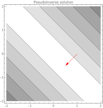
sol2={1,1}.PseudoInverse[H];x0={1,0};Show[plt,Graphics[{Red,Arrow[{x0,x0-sol2}]}],PlotLabel"Pseudoinverse solution"]
Out[]=
In[]:=
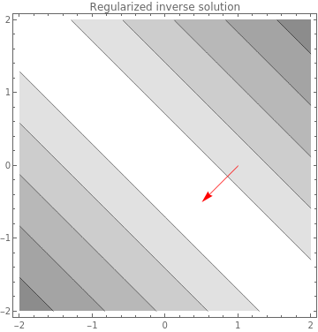
l=0.1;sol3={1,0}.Inverse[H.H+lIdentityMatrix[2]].Hx0={1,0};Show[plt,Graphics[{Red,Arrow[{x0,x0-sol2}]}],PlotLabel"Regularized inverse solution"]
Out[]=
{0.243902,0.243902}
Out[]=