An overview of the elementary statistics of correlation, R-squared, cosine, sine, and regression through the origin, with application to votes and seats for Parliament
An overview of the elementary statistics of correlation, R-squared, cosine, sine, and regression through the origin, with application to votes and seats for Parliament
Thomas Colignatus
February 20 2018 - version and update in Mathematica April 9 & 16 2018
February 20 2018 - version and update in Mathematica April 9 & 16 2018
Abstract
Abstract
The correlation between two vectors is the cosine of the angle between the centered data. While the cosine is a measure of association, the literature has spent little attention to the use of the sine as a measure of distance. A key application of the sine is a new “sine-diagonal inequality / disproportionality” (SDID) measure for votes and their assigned seats for parties for Parliament. This application has nonnegative data and uses regression through the origin (RTO) with non-centered data. Textbooks are advised to discuss this case because the geometry will improve the understanding of both regression and the distinction between descriptive statistics and statistical decision theory. Regression may better be introduced and explained by looking at the angles relevant for a vector and its estimate rather than looking at the Euclidean distance and the sum of squared errors. The paper provides an overview of the issues involved. A new relation between the sine and the Euclidean distance is derived. Equal or Proportional Representation (EPR) scales down from electorate to Parliament while District Representation (DR) confuses elections with contests (USA, UK).
Keywords
Keywords
general economics, social choice, social welfare, election, parliament, party system, representation, sine diagonal inequality / disproportionality, SDID, proportion, district, voting, seat, Euclid, distance, cosine, sine, Gallagher, Loosemore-Hanby, Sainte-Laguë, Webster, Jefferson, Hamilton, largest remainder, correlation, diagonal regression, regression through the origin, apportionment, disproportionality, equity, inequality, Big Data, Brexit, political science
Classifications
Classifications
MSC2010
62J20 Statistics. Diagnotics
00A69 General applied mathematics
28A75 Measure and integration. Length, area, volume, other geometric measure theory
97M70 Mathematics education. Behavioral and social sciences
JEL
A100 General Economics: General
D710 Social Choice; Clubs; Committees; Associations,
D720 Political Processes: Rent-seeking, Lobbying, Elections, Legislatures, and Voting Behavior
D630 Equity, Justice, Inequality, and Other Normative Criteria and Measurement
©Thomas Cool, CC BY-NC-ND 4.0, https://creativecommons.org/licenses/by-nc-nd/4.0/
Version in Mathematica
Version in Mathematica
The original version of this paper is Colignatus (2018e) at MPRA. It seemed useful to make a version in Mathematica as well. The packages used in Colignatus (2018a) are included here again to create Figure 1. A small utility package is included for this present version as well for an improved Figure 2. Typing errors have been corrected and at some points clarity has been enhanced. Footnotes have become endnotes. The reference to McShane et al. (2017) has been included. This present version is also available in the cloud, see http://community.wolfram.com/groups/-/m/t/1317181 and its attachment.
Contents
Contents
1. Introduction 1.1. The subject of discussion 1.2. Votes and seats 1.3. Structure of the paper 2. Notation and basics 2.1. Well-known basics 2.2. Regression through the origin (RTO), for nonnegative vectors2.3. A view from didactics3. Evolving statistics 3.1. The statistical triad of Design, Description and Decision3.2. A possible reason why RTO may be less prominent in the textbooks 3.3. Statistical significance 3.4. Causality 3.5. Specification search 4. Application to votes and seats 4.1. Descriptive statistics and decisive apportionment 4.2. Different worlds for votes and seats: DR and EPR 4.3. Apportionment in EPR 4.4. Different models and errors 4.5. Disproportionality, dispersion and education 4.6. True variables v* and s* and particular observations v and s 4.7. Cos, slope and concentrated numbers of parties (CNP) 4.8. Analyses of squares for the direct error 4.9. Symmetry 5. More on interpretation 5.1. Statistics and heuristics on the slope 5.2. Electoral justice and inequality 5.3. From the Humanities to Science 5.4. The example of Brexit 6. Conclusions 7. Footnotes 8. References
Start (evaluate this subsection for the initialisation packages)
Start (evaluate this subsection for the initialisation packages)
1. Introduction
1. Introduction
1.1. The subject of discussion
1.1. The subject of discussion
Karl Pearson (1857-1936) designed correlation between two vectors with the deliberate focus on centered data, namely to capture as much variation as possible. This arrangement also applied to the coefficient of determination, or R-squared, between a vector and its estimate.
2
R
We now have reason to look at the original and non-centered data, and in particular at nonnegative data. This application arises for votes and the assigned seats for parties for Parliament. When we want equal proportions of votes and seats, or to maximise the association, or to minimise the inequality / disproportionality (ID), then it would not make sense to center the data. Having a vector of seat shares at a constant distance of a vector of vote shares would be rather curious. For such non-centered data we apply regression through the origin (RTO), see Kozak & Kozak (1995) and Eisenhauer (2003). Textbooks tend to warn against dropping the constant in the regression, since it is better to test whether modeling errors show up in an estimated constant, yet in this case RTO appears to be the proper approach.
Obviously, both Pearson’s centered data and RTO share the property that the constant is zero, yet remarkably there are some differences for nonnegative data. This article will use this framework of nonnegative vectors, following Colignatus (2017ab) (2018abcd), but potentially some properties might be generalised for other data.
Pearson also concentrated on the cosine as a measure of similarity. The literature has spent little attention to the use of the sine as a measure of distance. For shares of votes and seats one might say that they are 97% close but the literature had focussed on developing measures of inequality / disproportionality, as people might be more sensitive to the 3% dissimilarity. Colignatus (2018d) discusses measures for votes and seats, and develops the new sine-diagonal inequality / disproportionality (SDID) measure. SDID uses not only the sine but also the square root on the sine, as a magnifying glass for small values, like the logarithm in the Richter scale. Colignatus (2018a) gives a more general perspective on distance and norm, and rejects the Aitchison geometry for compositional data for this comparison of votes and seats. [1] There are particular aspects in voting, like majority switches, that are not relevant for other applications. The sine measure is more sensitive than the angular distance, and also interesting since it links up to regression, since finds its translation in RTO as the squared cosine of the angle between the vectors. A new finding in Section 4.8 below is a direct relation between the sine and the Euclidean distance between two vectors.
2
R
Our objective here is to provide an overview of the elementary statistics of correlation, R-squared, cosine, sine, and regression through the origin (RTO), with application to votes and seats for Parliament. While our focus is on the relevance for statistics, with an eye on education in statistics, [2] we cannot avoid highlighting aspects of votes and seats, since this content determines the analysis. For earthquakes there exists the Richter scale, but for votes and seats there isn’t yet a similar “change” measure, while the advice now is to use SDID.
We will look at the same issue from different perspectives (statistics versus the issue of content on electoral systems, correlation versus trigonometry, theory versus education) and thus cannot avoid repetition, which however helps to identify that we are speaking about the same issue.
We use x for a real vector, and ||x|| = for the norm of x, and ||y - x|| for the Euclidean distance between x and y. Normalised are x* = x / ||x|| and y* = y / ||y||. There is also θ for the angle between x and y. Linear algebra provides an expression for the cosine of this angle, as Cos[x, y] = x'y / = x*’y*, i.e. the improduct of the normalised vectors on the unit circle. Cos is essentially the projection divided by the radius 1, see also the discussion and graph below. [3] Then θ = ArcCos[Cos[x, y]]. The formula for the cosine is scale invariant, as the angle does not change for positive scalars λ and μ, with Cos[x, y] = Cos[λ x, μ y].
x'x
x'xy'y
1.2. Votes and seats
1.2. Votes and seats
Let v be a vector of votes for parties and s a vector of their seats gained in the House of Commons or the House of Representatives. We discard zeros in v and use a single zero in s for the lumped category of "Other", of the wasted vote, for parties that got votes but no seats. Let V = 1'v be total turnout and S = 1's the total number of seats, and w = v / V and z = s / S the perunages. For presentation we will use 10 w and 10 z and the range [0, 10] in general. For votes and seats, percentages [0, 100] generate too much an illusion of precision, while [0, 1] generates too many leading zeros. Distance measures on [0, 10] read as an inverted (Bart Simpson) report card (with much appreciation for a low score). [4]
In political science, the main current inequality / disproportionality (ID) measures are (conventionally for percentages but now with 10): [5]
◼
Absolute difference / Loosemore-Hanby (ALHID): 10 Sum[Abs[z - w] / 2]. The division by 2 corrects for double counting. An outcome of 1 means that one seat in a House of] 10 seats is relocated from equality / proportionality.
◼
Euclid / Gallagher (EGID): 10 . For two parties this equals ALHID.
Sum2
2
(z-w)
◼
2
Χ
2
1)
2
w)
Sum(z/w-1)2
2
2
w
◼
The difference in shares for the “largest” party, i.e. with the most seats: 10 - ). This is an easy, rough and ready indicator with some history in the literature, and Shugart & Taagepera (2017:143) show remarkably that EGID ≈ 10 - ).
(
z
L
w
L
(
z
L
w
L
The proposed new sine-diagonal inequality / disproportionality (SDID) measure has the formula SDID[v, s] = sign 10 . The sine is invariant to scale: Sin[v, s] = Sin[w, z]. With k = Cos[v, s] given by linear algebra, we might use θ = ArcCos[k] and then find Sin[v, s] = Sin[θ] but we can also use Sin[θ] = directly. The additional square root on Sin works as a magnifying glass for inequalities / disproportionalities. The sign indicates majority switches, and is 1 for zero or positive covariance and -1 for negative covariance. [6] ALHID and EGID have a division by 2 to remain in the [0, 10] range, while Sin achieves the same purpose without such division. The newly derived relation in Section 4.8 explains this.
Sin[v,s]
1-
2
k
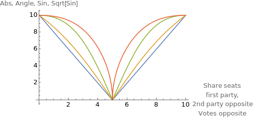
To clarify the distinction between the new proposal and the conventional measures in political science, Figure 1 gives ALHID (blue) and SDID (red), and the intermediate steps given by the angle (yellow) and sine itself (green). [7] For two parties normalised to [0, 10] we plot with seats = {t, 10 - t}, with t the seats for the first party. We also consider opposite values votes = {10 - t, t} = 10 - seats. Since this implies negative correlation, the SDID becomes negative, but the plot gives the absolute value. To wit:
◼
The angular measure (AID) is 10 θ / 90° (yellow), Since we look at nonnegative vectors, the maximum angle is 90°.
◼
The sine plotted is 10 Sin[θ] (green). For small angles there is little difference between Sin[θ] and θ in radians. There is a large difference between Sin[θ] and θ / 90°.
The key point of Figure 1 is that the SDID indeed works like a magnifying glass to determine inequalities / disproportionalities in votes and seats. This relates to the Weber-Fechner law on psychological sensitivity. [8] When a frog is put into a pan with water at room temperature and subsequently is slowly boiled it will not jump out. When a frog is put into a pan with hot water it will jump out immediately. People may notice big differences between vote shares and seat shares, but they may be less sensitive to small differences, while these differences actually can still be quite relevant for the decision to jump out. For this reason, the SDID uses a sensitivity transform. Like with the Richter scale, it will now be easier to relate the smaller values to the larger values. At the values t = 4.5 or 5.5, when the absolute distance ALHID registers a 1 on a scale of 10, SDID generates a staggering 4.4 on a scale of 10, which outcome better relays the message that this difference is alarming.
Figure 1. Plot of d[votes, seats] for votes = 10 - seats and seats = {t, 10 - t},
for d = Abs/2, AngularID, Sine, and |SDID| (eliminating the latter’s negative sign)
for d = Abs/2, AngularID, Sine, and |SDID| (eliminating the latter’s negative sign)
As another example: When votes {4.9, 5.1} are translated into seats then the absolute difference (ALHID) and the Euclidean distance (EGID) regard outcomes {4.8, 5.2} or {5.0, 5.0} as at the same distance, namely 0.1 seat difference (correcting for double counting), while common sense and the sine would hold that the seats {4.8, 5.2} are closer to the votes and less disruptive than the seats {5.0, 5.0} that suggests that there is equality. The values are: 10 Sin[{4.9, 5.1}, {4.8, 5.2}] = 0.1998 < 0.19996 = 10 Sin[{4.9, 5.1}, {5.0, 5.0}]. [9] These values are so close together, though, that also the magnifying glass SDID hardly sees a difference: 1.41351 < 1.41407. However, the latter values are still at the high level or 1.4 on a scale of 10, rather than at the low value of 0.1 on a scale of 10 for ALHID. [10]
Table 1 contains the real world example of the US House of Representatives of 2016 (435 seats) and the UK House of Commons 2017 (650 seats). SDID properly conveys the insight that there is shocking inequality / disproportionality.
Table 1. Votes and seats in the USA 2016 and UK 2017 [11]
USA | 2016 | S=435 | UK | 2017 | S=650 | |
Party | Votes | Seats | Party | Votes | Seats | |
Republicans | 4.91 | 5.54 | Conservatives | 4.22 | 4.88 | |
Democrats | 4.80 | 4.46 | Labour | 3.99 | 4.03 | |
Other | 0.29 | 0 | Other | 1.79 | 1.09 | |
100% | 10 | 10 | 100% | 10 | 10 | |
10( z L w L | 0.63 | 10( z L w L | 0.66 | |||
ALHID | 0.63 | ALHID | 0.70 | |||
AID | 0.67 | AID | 0.92 | |||
SDID | 3.2 | SDID | 3.8 |
1.3. Structure of the paper
1.3. Structure of the paper
The square root within SDID is psychologically important and only a presentation feature of descriptive statistics. This present discussion collects the key steps in Colignatus (2018d) for the content of statistics and targets at an overview. Part of the present text has already been used on my weblog Colignatus (2017b).
The next section provides notation and basics. The subsequent section places our topic within the perspective of the statistical triad of experimental design, description and decision. Subsequently we apply the cosine and sine for nonnegative data, and state the relevant formulas. We close with a summary of the findings.
The reader might be advised to peek at Table 2 for a glance at the different models, to see what this discussion is about specifically. I have considered putting this table up front, but it remains better to first rekindle awareness about the basics before delving into the models.
PM 1. See Colignatus (2007) for the approach with determinants rather than angles - as area and volume might generalise easier to more dimensions than the angle, that might remain stuck to the 2D plane created by the two vectors. PM 2. There is also the notion of “distance correlation” [12] but the Pearson correlation remains relevant here precisely because of the linearity contained in the notion of equality / proportionality. PM 3. There is “least angle regression” [13] but such is different, and we remain in the realm of “simple regression”. [14]
2. Notation and basics
2. Notation and basics
2.1. Well-known basics
2.1. Well-known basics
We use the underlined upper case X for the centered value X = x - . The angle θ* is between the centered values X and Y. The Pearson correlation coefficient is r[x, y] = Cos[x - , y - ] = Cos[X, Y] = Cos[θ*] so that θ* = ArcCos[r[x, y]]. The covariance of x and y is the improduct of the centered values, divided by the number of observations n, or cov[x, y] = X' Y / n. Using covariance, the correlation coefficient r[x, y] = cov[x, y] / . See e.g. Egghe & Leydesdorff (2009) for a visualisation of the shift towards centered data, and Theil (1971:165) for a discussion of the geometric meaning that r = Cos[θ*].
x
x
y
cov[y,y]cov[x,x]
Along (1) θ and (2) θ*, we also consider the linear cases of (3) the “regression through the origin” (RTO) for y given x, without a constant, (4) the “regression” in general, with a standard constant, hence for Y given X. For linearity, the standard case with a constant may also be formulated in terms of y and x, but some formulas then require the mention of the means. The symbol ŷ will be the estimate of y, but e and ê are just different kinds of error.
For (4) with centered Y = X b + ê for matrix X, then Y'Y = b'X'X b + ê'ê using X'ê = 0. This is commonly expressed as SST = SSX + SSE. In this, Y'Y = SST = sum of squares total, ê'ê = SSE = sum of squared errors, and SSX = sum of squares of the explanation = SST - SSE. [15]
The coefficient of determination is = SSX / SST. Thus 1 - = SSE / SST. For the calculation of SST and SSE we must use centered data, though the regression itself might also be formulated as y = X b + ê with a column of 1 in X for the constant. With n observations and m explanatory variables in X, the root mean squared error (RMSE) adjusted for the degrees of freedom is RMSE = . Colignatus (2006) discusses the sample distribution of (adjusted) R-squared. When the (explanatory) variables are given without measurement errors then there is not a “population” but a “space”, and the relevant parameter for R is best denoted as ρ[X] to express the conditionality on the data.
2
R
2
R
SSE/(n-m)
The angle itself is a measure of distance. The angle divided by 360° gives a measure in [0, 1]. See Colignatus (2009, 2015) for a suggestion to measure angles on [0, 1] anyway, using the plane itself as the unit of account, and to speak about turns. When it doesn’t matter whether the angle is positive or negative, then 180° would be a relevant maximum. For nonnegative data the relevant maximum is 90°. Subsequently 1 minus such value is an angular measure of association.
2.2. Regression through the origin (RTO), for nonnegative vectors
2.2. Regression through the origin (RTO), for nonnegative vectors
At stake now is the use of θ of the original and non-centered vectors, which leads us to regression through the origin (RTO). Also, we consider nonnegative vectors. In this case, the angle between the vectors is between 0 and 90°.
There are slopes b and p from the regressions through the origin (RTO) z = b w + e and w = p z + ε. Then k = Cos[v, s] = Cos[w, z] = Sqrt[b p]. The geometric mean slope is a symmetric measure of similarity of the two vectors. Also Sin[v, s] = Sin[w, z] = Sin[θ] = Sqrt[1 - b p] is a metric and a measure of distance or inequality or disproportionality in general.
All this is straightforward but there are some reasons to call attention to it.
◼
Political scientists have been looking for a sound inequality / disproportionality measure without finding one, i.e. not finding the sine. They have been setting for the less adequate Euclidean distance EGID discussed (not proposed) by Gallagher (1991), though with an awareness that it wasn’t perfect, see Taagepera & Grofman (2003), Karpov (2008) and Koppel & Diskin (2009). Colignatus (2018 d) provides an overall evaluation.
◼
The use of angle, cosine and sine gives a perspective on compositional data (i.e. nonnegative values on the unit simplex), see Barceló-Vidal and Martín-Fernández (2016). This is discussed in Colignatus (2018 a). Votes and seats are somewhat special data however. Seats don’t fall from the sky and tend to be apportioned given the votes and the available seats in the House, as ŝ = Ap[S, v]. This means that the influence of S cannot be neglected as perhaps may be done in “pure” compositional data.
◼
Compositional data generally would use a log transform (with the geometric average as the mean) and drop one equation because of the addition condition. For the present paper, however, we don’t employ statistical decision theory, with regression as one of its applications, but we employ statistical description (without distinction between true coefficient b and its estimate). For determination of the angle between the vectors all elements are relevant, though still with the scalar invariance. Seeming "compositional data" like votes and seats contribute to our understanding of RTO that we consider two errors, not only z = b w + e (used by SDID) but also z = w + ẽ (used by ALHID, EGID and relatively by CWSID).
However, a binary regression in RTO has y = b x + e and ŷ = b x, so that Cos[y, ŷ] = Cos[y, x] because of scale invariance, so that the angle is fixed. We still require another criterion than the angle on y to find the parameter b.
◼
From y = b x + e we can also take the improduct x’y = b x’x + x’e, and set x’e = 0, so that b = y’x / x’x. This is shorter but requires geometry instead of calculus.
The latter approach projects y onto x and imposes perpendicularity between x and e, so that Cos[x, e] = Cos[x, y - b x] = 0 which gives x'e = 0. The projection of y on x is given by b x, with b = x'y / x'x, using projection matrix P = x x' / x'x and P y = b x. At this value of b the length of e is smallest. Taking the shortest distance is equivalent to minimising ||e|| but the geometry avoids the calculus. Figure 2, taken from Colignatus (2011:143), shows the geometry how y is projected onto x, which determines the size of the Explanation (b x), so that Effect y follows from addition of perpendicular Cause b x and Error e. On he LHS Cause and Effect are normalised onto the unit circle, so that the coefficient is Cos or R at 63%. The RHS is not normalised with coefficient b = 0.546. [In this version of the paper, the LHS has been clarified with the arcs at radius 1 and at radius 0.63.]
Thus there is a geometric approach that is at least as intuitive as the minimisation of SSE with reference to the normal distribution. The conceptual link between perpendicular x and e and minimal SSE need not be intuitive however, and can only be proven exactly by looking at the normal equation.
Both approaches generate the same solution, and there is only the difference in presentation, either via the angles between the vectors or the Euclidean norm of the error. Both relate to the assumption of i.i.d. normal errors, but the latter can also be seen as step 2, when one agrees that it is more informative to start with the use of the angle as step 1, rather than derive the angle as a corollary or be actually silent on it.
My suggestion is that the world of statistics develops a greater awareness of the angle and sine as distance metrics in relation to R-squared, at least for applications of RTO for such nonnegative data. For textbooks in statistics, this particular combination might be regarded as a missing link. The geometry would contribute to a better understanding of students of both regression and the distinction between descriptive statistics (no distinction between b and an estimate) and statistical decision theory (a true b and its estimate).
2.3. A view from didactics
2.3. A view from didactics
In education it happens far too often that a textbook starts a new section with “Now something completely different” while it appears that one essentially has the same topic though only from another perspective. Consider for example {x, y} = x + y = r (Cos[φ] + Sin[φ]) = Exp[r + φ]. Or, in fact, that above shortest distance can be found by both projection and calculus, creating the field of analytic geometry. Obviously such perspectives exist and each perspective has something to say for it, and obviously it is a result in itself when one can show the equality. But one also feels rather exasperated, finding out that one only learns different languages for the same.
In the same way for correlation. The “explanation” on correlation, that “correlation between two vectors is the cosine of the angle between the centered data”, is only required because the word “correlation” has been introduced without explicit reference to the basic angularity of the notion. Most students, who first are introduced to “covariance” and who then are presented with correlation by a formula that uses covariance, will miss out on the notion that correlation refers to an angle. Even when this is derived it tends to remain a mystery because students have built up mental maps on “correlation” that tend to be quite different from angles.
It would be preferable to first set up the basic structure of correlation and regression in this clean manner, before entering upon the error distribution, such that “mean” is replaced by “expectation”, and with such use of covariance. Present textbooks (curriculum) however shy away from re-engineering trigonometry, and work around corners by introducing correlation as if it were something really new. In practice they block the understanding by many.
3. Evolving statistics
3. Evolving statistics
3.1. The statistical triad of Design, Description and Decision
3.1. The statistical triad of Design, Description and Decision
Statistics has the triad of Design, Description and Decision. Up to fairly recent, statistics relied much upon the paradigm by R.A. Fisher that focused on population and sample distributions. With the dictum “correlation is not causation”, statistics assumed that causation was given by the scientific model, and then concentrated on correlation for cases with clear causality. Since Pearl (2000), the issue of causality is more in focus again, though this doesn’t change the triad.
◼
Design is especially relevant for the experimental sciences. Design is much less applicable for observational sciences, like macro-economics and national elections when the researcher cannot experiment with nations.
◼
Descriptive statistics has measures for the center of location - like mean or median - and measures of dispersion - like range or standard deviation. Important are also the graphical methods like the histogram or the frequency polygon. Measures like the Richter scale for earthquakes belong in this category too. Description relates to decisions on content (e.g. in medicine or economics). Description becomes more important because of Big Data.
◼
Statistical decision making involves the formulation of hypotheses and the use of loss functions to choose alpha and beta values to evaluate hypotheses. A hypothesis on the distribution of the population provides an indication for choosing the sample size. A typical example is the decision error of the first kind, i.e. that a hypothesis is true but still rejected. The probability of that error, the alpha, is called the level of statistical significance. This notion of statistical significance differs from causality and decisions on content. (See e.g. Varian (2015).)
Historically, statisticians have been working on all three areas, but the most difficult was the formulation of decision methods, since this involved both the calculus of reasoning and the more involved mathematics on normal, t, chi-square, and other frequency distributions. In practical work, the divide between the experimental and the non-experimental (observational) sciences appeared insurmountable. The experimental sciences have the advantages of design and decisions based upon samples, and the observational sciences basically rely on descriptive statistics. When the observational sciences do regressions, there may be an ephemeral application of statistical significance that invokes the Law of Large Numbers, that all error is approximated by the normal distribution.
This statistical tradition is being challenged by Big Data including the ease of computing - see also Wilcox (2017). When the relevant data are available, and when you actually have the space or population data, then the idea of using a sample may evaporate, and you would not need to develop hypotheses on those distributions anymore. In that case descriptive statistics tends to become the most important aspect of statistics. Decisions on content then are less compounded by statistical decision making on statistical phenomena. It comes more into focus how descriptive statistics relate to decisions on content. Such questions already existed for the observational sciences like for macro-economics and national elections, in which the researcher only had descriptive statistics, and lacked the opportunity to experiment and base decisions upon samples. The disadvantaged areas may now provide insights for the earlier advantaged areas of research.
The suggestion is: to transform the loss function into a descriptive statistic itself. An example is the Richter scale for the magnitude of earthquakes. A measurement on that scale is both a descriptive statistic and a factor in the loss function. A community making a cost-benefit analysis has on the one hand the status quo with the current risk on human lives and on the other hand the cost and benefit of investments in new building and construction including the risk of losing the investments and a different estimate on human lives. In the evaluation, the descriptive statistic helps to clarify the content of the issue itself. For the amount of destruction it would not matter how earthquakes are measured, but for human judgement it would, as the human mind need not be sensitive to relevant differences. The key issue is no longer a decision within statistical hypothesis testing, but the key issue is the adequate description of the data and the formulation of the decision problem in terms for better human understanding of what is involved.
3.2. A possible reason why RTO may be less prominent in the textbooks
3.2. A possible reason why RTO may be less prominent in the textbooks
Statistics and specifically textbooks apparently found relatively little use for original (non-centered) data and RTO. A possible explanation is that statistical theorists fairly soon regarded descriptive statistics as less challenging, and focused on statistical decision making. Textbooks prefer the inclusion of a constant in the regression, so that one can test whether it differs from zero with statistical significance. The constant is essentially used as an indicator for possible errors in modeling. The use of RTO or the imposition of a zero constant would block that kind of application. This (traditional, academic) focus on statistical decision making apparently caused the neglect of a relevant part of the analysis, that now comes into focus again.
3.3. Statistical significance
3.3. Statistical significance
Part of the history is that R.A. Fisher with his attention for mathematics emphasized precision for statistical purposes while W.S. Gosset with his attention to practical application on content emphasized the effect size of the coefficients found by regression. Somehow, precision in terms of statistical significance became more important in textbooks than content significance. Perhaps the simple cause is that statistical manuals focus on what statistics can do, while they leave it to the fields of application to focus on the effect sizes. When the fields of application ask for advice on statistics, this is what they get, yet they should not forget about their own task on the effect sizes. Empirical research has rather followed Fisher than the practical relevance of Gosset. This history and its meaning is discussed by Ziliak & McCloskey (2007), see also the discussion by Gelman (2007) referring to Gelman & Stern (2006), and McShane et al. (2017).
3.4. Causality
3.4. Causality
3.5. Specification search
3.5. Specification search
4. Application to votes and seats
4. Application to votes and seats
4.1. Descriptive statistics and decisive apportionment
4.1. Descriptive statistics and decisive apportionment
Vectors s and z = s / s'1 have been created by human design upon v, and not by some natural process as in common statistics. A statistical test on s | v would require to assume that seats have been allocated with some probability, and this doesn’t seem to be so fruitful when there was an underlying system of rules. We can use the same linear algebra however, now for descriptive statistics.
The ID measures are used to compare outcomes of electoral systems across countries, though such comparisons have limited value when countries have different designs. Taagepera & Grofman (2003) mention also some other reasons for an ID measure: (i) comparison on President, Senate, House, or regional elections (what they call "vote splitting" but is better called: votes for different purposes), (ii) comparison on years in similar settings (both votes and seats) (what they call "volatility" but what is better called: votes on different occasions).
Above measures ALHID, EGID and CWSID have drawbacks and are inoptimal. There appears to be some distance between the voting literature on inequality / disproportionality and the statistics literature on association, correlation and concordance. A main point is that voting uses ẽ = z - w (conventionally) and now we focus on z = b w + e (for SDID) as descriptive, while statistical theory tends to think in terms of hypotheses tests on general relationships like s = c + B v + u and then requires stochastics.
4.2. Different worlds for votes and seats: DR and EPR
4.2. Different worlds for votes and seats: DR and EPR
A general distinction is between District Representation (DR) and Equal or Proportional Representation (EPR). “Elections” in systems of EPR differ from those in DR, and we should actually avoid the single term “election” for both cases when the meanings are fundamentally different, see Colignatus (2018c).
◼
EPR recognises that elections for Parliament concern multiple seats, such that there are conditions for overall optimality.
◼
DR has district elections that neglect conditions for overall optimality. Each district may have a number of seats, called the district magnitude M, and generally M ≪ S. In single seat districts (SSD), M = 1, the district vote for a Member of Parliament is treated as a single seat election, say comparable to the vote for the US President.
EPR concerns proper election of representatives for Parliament, with the clear purpose to scale the electorate down to the size of Parliament. DR can better be diagnosed as a contest. In DR, votes for candidates other than the district winner(s) are not translated into seats, and the system discards those votes. DR-elections have much strategic voting for fear that the vote is lost. The true first preferences thus are masked. Comparing votes and seats is comparing masked votes and actual seats, with often unknown discarded votes. Only geography might cause a semblance of balancing at the national level. Also the median voter theorem might cause that voters concentrate around the middle, but this should not deceive us in thinking that we could achieve a proper "comparison" of votes and seats in DR. Table 1 concerns countries with DR, and the scores of the ID measures are on masked data, and we may well have "garbage in, garbage out". We will return to this issue on content below, including the confusions that a contest scales down too, and that each election would also be a contest.
4.3. Apportionment in EPR
4.3. Apportionment in EPR
Only in EPR there is a deliberate apportionment of the seats given the votes, with s = ŝ = Ap[S, v].
◼
In general the apportionment will not be perfect, since the distribution over perhaps millions of votes must be approximated by perhaps a few hundred seats (with integer values). The apportionment involves some political philosophies that have been adopted by the national parliaments.
◼
There need not be a real distance between the voting literature and statistics, at roots, because (i) the Chi-Square / Webster / Sainte-Laguë (CWSID) apportionment philosophy obviously compares with the Chi square, and (ii) the apportionment according to Hamilton / Largest Remainder (HLR) minimises the absolute difference, or the Loosemore-Hanby index (ALHID), but also minimises the sum of squared differences, or the Euclidean distance (or the EGID index). Perhaps this early historical linkage also caused the presumption that voting theory already “had enough” of what was available or relevant in the theory of statistics.
◼
Researchers on voting may have a tendency to remain with these philosophies when they measure the outcomes from such apportionments too. Apportionment (deciding) and measuring (describing) have different purposes and methods tough, even while there may be a family resemblance.
◼
When comparing results from different countries, however, it would make sense, to use a common best measure, rather than reporting that each country applies its own method.
There are more aspects, yet this present article does not focus on voting theory but on giving an overview of statistics, that is also applicable for this setting. The present discussion however highlights where comparing votes and seats differs from other purposes in statistics: (i) First the requirement on the diagonal of the scatter plot of w and z. (ii) Secondly, comparing votes and seats cannot rely on stochastic assumptions for testing, and thus wants to describe & measure. We use the same linear algebra but for a different purpose. The discussion helps to see that the choice of an inequality / disproportionality measure apparently is not self-evident, at least with the current literature and textbooks so dispersed over the topics that come together here.
4.4. Different models and errors
4.4. Different models and errors
We do not want to explain s by v, in which case we would be very careful w.r.t. the exclusion of the constant. Instead, we want to design a measure. This still uses the same linear algebra. The relevant distinctions are (i) between true values versus observations (with errors) or estimates, and (ii) between level variables versus unitised variables.
Q = V / S is the natural quota, or number of votes to cover a seat. There may be a threshold to get a seat, or just the natural quota. Voters may vote for parties that do not pass the threshold and that thus get no seats. This sums to the “wasted vote” W. Standardly the wasted vote and zero seats are collected in one category “Other”, so that v and s still have the same length. The votes that cause a seat are Ve = V - W. For regression it is conventional to write s = T v, so that s is explained by v. We call this vector-proportionality because of the lack of a constant. Any such relation also holds for its sum totals, and we can usefully define T = S / V = 1 / Q. In reality we have s = B v + u or z = b w + e with proportionality parameter b and error e. There is only unit proportionality or equality if z = w or b = 1 and e = 0. Let a = S v / V = T v = v / Q = S w be the proportionally accurate average of seats that a party might claim. A common error term is (s - a) = S (z - w). There will be at least an error from the need of integer values for seats. The value a = S w will be the average, and apportionment of s will tend to be for Floor[a] ≤ s ≤ Ceiling[a]. The major distinctions are in Table 2.
Table 2. Basic models and their errors
The analysis better uses regresssion through the origin (RTO) and not regression with a constant (Pearson). The unit simplex is the natural environment to look at this, though we should not forget about the role of S. There are three different error measures:
◼
ê from the standard regression with a constant, using centered data (Pearson).
◼
e from RTO, with coefficient b = z'w / w'w. (SDID uses e.)
◼
ẽ = z - w or the plain difference, using b = 1. (ALHID and EGID use ẽ.)
Some useful mnemonics directly are:
1
.ê'ê ≤ e'e ≤ ẽ'ẽ because regression parameters allow the reduction of error.
2
.e picks up a potential source for proportionality that ẽ does not allow for.
3
.1'ẽ = 0 and b = 1 - 1'e because 1'z = 1'w = 1.
4
.b = z'w / w'w because we multiply z = b w + e with w' while w'e = 0. The regression selects the b with perpendicular w and e, or with w'e = 0 and minimal e'e.
5
.Taking the plain differences ẽ = z - w and weighing them by the vote shares and normalising on their squares, gives w'ẽ / w'w = b - 1 (= -1'e from above). This b = 1 + w’ẽ / w’w might perhaps be seen as an “implicit outcome”, though it only works of course since we already identified b from geometry.
4.5. Disproportionality, dispersion and education
4.5. Disproportionality, dispersion and education
The notion of “proportionality” derives from the notion that the seats (tens) for the parties should be proportional to the votes (millions) for the parties. A formal statement is s = T v. When we shift attention to
the shares w and z then we want these proportions to be equal. We run a bit into a verbal complication when we want to see that w and z would be proportional too.
the shares w and z then we want these proportions to be equal. We run a bit into a verbal complication when we want to see that w and z would be proportional too.
For education we want to maintain that we want to explain to students that any line through the origin in 2D represents a proportional relationship. For vectors and their scatter plot we would speak about "vector-proportionality". Thus, also for z and w, a relation z = α w is a vector-proportional relationship, and z = w is only unit or diagonal vector-proportional. It so happens that the unit simplex is defined such that 1'z = α 1'w, thus any pure proportional relation in that space requires a = 1 of necessity. I would phrase this as that the space is defined such that those other pure vector-proportions do not exist. I would not phrase it as saying that (quote) "z = α w for α ≠ 1 would not be vector-proportional and that only α = 1 is vector-proportional" (unquote). It is better to say: “We only have z = b w + e with vector-proportionality parameter b and scattered e.” Thus, overall, it would be didactically preferable to speak about "unit or diagonal proportionality" for voting rather than "proportionality". Only when e = 0 then we also have equality. Equal Representation is better anyway, when I abbreviate EPR instead of PR. It may be difficult to change a convention, but it would help for mathematics education.
This calls attention to the relation with dispersion. Table 3 reviews the relations. The key relationship in RTO is that b = 1 - 1'e. Thus b = 1 ↔ 1'e = 0. The upper right cell is impossible: Not[e = 0 & 1'e ≠ 0]. The lower right case of disproportionality implies dispersion, but dispersion (e ≠ 0) need not imply such disproportionality. The middle column with b = 1 is in opposition to the right column, but we must distinguish between unit or diagonal vector-proportionality without dispersion (equality) and average unit or average diagonal vector-proportionality with dispersion.
Table 3. Disproportionality and dispersion in Regression Trough the Origin
(RTO)
(RTO)
With b = 1 then e = z - b w = z - w = ẽ. We already had 1'ẽ = 0 but b = 1 causes also 1'e = 0. With b = 1 then w'(z - w) = 0, of which z - w = 0 is only a special case.
4.6. True variables v* and s* and particular observations v and s
4.6. True variables v* and s* and particular observations v and s
A proportional relationship for 1D variables is best described by the 2D line λ y + μ x = 0, which coefficients may be normalised on the unit circle. For nonzero λ this reduces to y = T x with T = - μ / λ, where slope T also is the tangent of the angle of the line with the (horizontal) x-axis. For vectors this generalises into vector-proportionality, with now a plane u = λ y + μ x and then choosing u = 0 so that y = T x again. For example, y = {1, 2, 3} and x = {2, 4, 6}, then T = ½, and we would see a line without dispersion in the scatter plot.
◼
The notion of unit proportionality as in the line y = 1 x + 0 is a mathematical concept, while in statistics with dimensions we can rebase the variables, so that there need not be a natural base for 1.
◼
For voting, there are natural bases in the individuals and seats. Larger parliaments may have more scope for a better fit. Still, normalisation onto the unit simplex makes sense.
◼
At first sight it is not clear where voting differs from other applications, say the ratio of 1 car per 2 persons. Any vector-proportional relation s = T v also holds for the totals. Thus S = 1's = T 1'v = T V. In {w, z} space it reduces to a scatter with diagonal z = w because division gives z = s / S = T v / S = w. When any vector-proportional relationship (also non-unity) is transformed onto the unit simplex, then they become unit or diagonal proportional in the scatter, and we lose the original information.
◼
There also is dispersion. For the sake of understanding this issue of proportionality, but not for the sake of estimation and hypothesis testing, we now distinguish true elements and their observations. The basic solution namely is to distinguish on one hand the true vector-proportionality s* = T* v* that holds for all true elements, and on the other hand observations (e.g. errors in variables) s = B V + u, for which we only have the definition for the sum totals as T = S / V. This also generates ũ from s = T V + ũ. For example for some v*, perhaps s* = a* = S w*.
◼
For theory we have z* = w* but for the data z = w b + e. We divided by S and took b = B V / S = B / T and e = u / S. Thus we should not focus only on parameters B and b but also be aware of the hidden Q = V / S or T = 1 / Q, and perhaps consider T as an estimate on T*.
4.7. Cos, slope and concentrated numbers of parties (CNP)
4.7. Cos, slope and concentrated numbers of parties (CNP)
For theory we have s* = T* v* for the vectors, but for the data we have s = B v + u and thus only T = S / V for the totals. Thus there are not only parameters B and b but also an “estimate” T on T* (or perhaps institutionally given T = T*). Table 4 reviews the relations. For readibility we drop the stars in the theory column on the LHS.
Table 4. Norm and estimation, in levels and unitised, regression through
origin (RTO)
origin (RTO)
Key points of RTO on the unit simplex are, using mostly the last column:
1
.The sum of errors 1'u or 1'e need not be 0, but 1' ũ = 0 and 1' ẽ = 0.
2
.It is a contribution to RTO by (seeming) compositional data that we now also look at T = S / V and s = T v + ũ, or z = w + ẽ. Voting theory currently uses this, but it might be inoptimal.
6
.v'u = w'e = 0, following the outcomes for B and b (or they are chosen such).
7
.The “analysis of squares” (no deviations and thus no “analysis of variance”) on SST gives:
9
.Thus there is a perfect fit e = 0 if and only if Cos = 1, when b = 1 and z = w.
10
.Observe that b = 1 - 1'e = B V / S = B / T = B Q so that B has a relevant dimensional factor.
13
.The footnote in the table is relevant unless you already saw the distinction between the columns, or the distinction between theoretical s* and v* and observed values s and v.
4.8. Analyses of squares for the direct error
4.8. Analyses of squares for the direct error
The interpretation of the RHS is: The sine makes the Euclidean distance ẽ' ẽ relative to z'z and subtracts a value h, because the cosine uses the slope to see proportionality that the Euclidean distance doesn’t pick up, and then rebases with this h to remain in [0, 1].
The deduction is:
4.9. Symmetry
4.9. Symmetry
(1) From w = w or z + q = p z + ε we find ε = q + (1 - p) z.
(2) With ε we have ε'ε = ε'q since z'ε = 0.
(3) With q we have q'ε = q'q + (1 - p) q'z = ε'ε because of (2).
(4) With z we get z'ε = z'q + (1 - p) z'z and with z'ε = 0: z'q = - (1 - p) z'z.
We already knew that both SDID and EGID are symmetric measures. That SDID picks up disproportionality from an implied slope b does not imply asymmetry (because of the asymmetry in the regression z = b w + e). The same sensitivity can also be formulated from the inverted regression.
The latter form can be rewritten using w* = w / ||w||. Then the relative sum of squared differences can also be seen as another weighted sum of relative differences:
5. More on interpretation
5. More on interpretation
5.1. Statistics and heuristics on the slope
5.1. Statistics and heuristics on the slope
This paper uses descriptive statistics, and we are not in hypothesis testing. The linear algebra in this paper should not be confused with statistical decision methods. The latter methods use the same linear algebra but also involve assumptions on distributions: and we will make no such assumptions. However, when the linear algebra results into a new measure, then this measure can be used for new statistics again.
Figure 3. Rubin’s Vase [25]
Alongside CWSID other common measures are the absolute difference / Loosemore-Hanby index (ALHID) and Euclid / Gallagher index (EGID). CWSID, ALHID and EGID are parameter-free, and clearly fall under descriptive statistics. My original view was that SDID is parameter-dependent, since it refers to b and p. Paradoxially, however, while we started out looking for a slope measure, Cos is actually parameter-free, since its value as a similarity measure can be found without thinking about slopes at all. It is just a matter of perspective, see Figure 3. Thus the bonus of above heuristic is only that it helps to better understand what the measure does. The awareness of this double nature is important for the comparison of ALHID and SDID. For ALHID one might argue that it takes error z - w = ẽ in Table 2 under the assumption that official regulations have chosen s = ŝ = Ap[S, v] with some optimality. Thus, the use of z = b w + e can be seen as changing the error. However, when Cos is regarded as a parameter-free measure of similarity, then no errors have been changed. Thus we can compare ALHID and SDID with this argument out of the way. Interpreting Cos as the outcome of RTO is only a bonus, that helps in the development of more perspectives. The useful perspective is that SDID may pick up more inequality / disproportionality than ALHID in the official s = ŝ = Ap[S, v] for example by an implied b that systematically differs from 1. And the cosine is a slope again in the equation with the standardised variables.
5.2. Electoral justice and inequality
5.2. Electoral justice and inequality
Balinski & Young (1976:2) quote Daniel Webster:
“To apportion is to distribute by right measure, to set off in just parts, to assign in due and proper proportion.”
Webster’s emphasis was on “due and proper” and not on “proportion”, but the world adopted “proportionality”. Arend Lijphart has written about proportionality as “electoral justice”. I have considered adopting the term “justice” too but settle for the notion that z = w means equal proportions, or equality. A 2D line y = ½ x is proportional too. Thus, rather than speaking about “proportionality” in comparing votes and seats, it is better to speak about unit or diagonal vector-proportionality and electoral equality. Similarly, while the standard expression is “Proportional representation” (PR) it would be better to speak about Equal or Proportional Representation (EPR) or even Equal Proportional Representation (EPR). I don’t think that there is much chance that the world will rephrase this for the sake of education, but at least it is important to explain the vocabulary as a possible source for confusion. [26]
5.3. From the Humanities to Science
5.3. From the Humanities to Science
The issue of votes and seats contains an awkward element. The issue merges a topic of content with methods of statistics, and it appears that political science can use an infusion from statistical ethics as well. For description we know that displaying squares by their heights is misleading, since comparing 5 and 10 is quite else than comparing 25 and 100. This principle also causes the need to magnify what might be overlooked though. Indeed SDID takes the square root of the sine again, similar to the logarithm of the Richter scale. The underlying issue however is much more involved.
The discussion in this section concerns the role of scientists as guardians of the quality of information. It is a normative issue whether EPR or DR is the “better” system. This is not at issue here. There is also a Baron von Münchhausen problem how voters are going to decide which system to adopt. We leave such issues aside, and concentrate on the quality of information. When (political) scientists provide statistics and research findings on “votes and seats” then the information should satisfy standards of science, and not play into confusions from common language. When the general public asks questions to scientists and when scientists provide answers, then the scientists should point out confusions in these questions, and clarify how answers from science can help avoid such confusions.
Colignatus (2018c) evaluates the “political science of electoral systems” and concludes that this branch of study still remains in the Humanities, without the methods of clear definitions, modeling and measuring as is required for proper Science. A telltale is the use of the word “election”, while EPR-elections (proper elections) are quite different from DR-elections (actually contests). The invitation to empirical scientists is to help re-engineer the “political science of electoral systems” to become a real science.
Remarkably, Shugart & Taagepera (2017), political scientists themselves, in a recommendable book that indeed is a major advance, tend to agree that “political science of electoral systems” in general isn’t a science yet indeed, and they present their own book as a rare exception: “Thus the book is a rare scientific book about politics, and should set a methodological standard for all social sciences.” (p:320) They point to the trap of testing for statistical significance and the direction of the coefficient, while neglecting the effect size that would be relevant on content. “This can produce valuable insights, but these so-called “empirical models” are not really models at all. (...) Every peasant in Galileo’s time knew the direction in which things fall - but Galileo felt the need to predict more than direction.” (p324).
Unfortunately, while S&T mention different properties of DR and EPR, and are aware, so to say, that “not all votes and seats are created equal” (an expression by Taagepera), they apparently are blind to the key distinction between elections and contests, and thus in this key respect they are widely off-track. [27] They employ the words “vote” and “seat” as if these would be sufficiently equal, while this is only superficially so. While we would expect that political scientists would understand what they are studying, apparently they don’t. And apparently it is necessary to belabour the point.
The above mentioned two possible confusions. The first is that contests also scale down from the electorate to Parliament. However, the very purpose and manner of scaling down are relevant. The second confusion is that all elections are contests in some respect. However, in EPR this “contest” would be on getting a larger share of the vote and hence a larger share of the seats, which quite differs from the contest of winning the largest share and then “winner takes all”. It is better not to change the meaning of the term “contest”, when it is used as a metaphor in comparing EPR and DR.
Let us focus on what “vote” and “seat” are about, and thus on what the term “representative” might mean. A common dictionary [28] emphasizes the legal meaning of “representative”. “2 a : standing or acting for another especially through delegated authority, b : of, based on, or constituting a government in which the many are represented by persons chosen from among them usually by election”. The dictionary also assumes that DR-elections and EPR-elections are all “elections” in a legal sense. Since direct democracy might only be feasible in town halls, we need representative democracy indeed, but the dictionary focuses on the legal setting and hides the key distinction between DR and EPR. As opposed to this common dictionary and legalistic thinking, in science we need strict definitions that fit the observations. We might make the assumption that the Moon is made of green cheese, but obviously we don’t. In a single seat case like for the President, one might argue that the President would represent the whole nation, but the House of Representatives has multiple seats, and this changes the logic of the case. Thus we get the distinction:
(1) In EPR, “representation” for Parliament means “standing for the people who have voted for you, by marking your name or party”. In EPR, a candidate gets a seat when the natural quota Q = V / S, the national average votes per seat, is covered, while this criterion is only lowered for the remainder seats. Thus there tends to be full backing by those like-minded, and this avoids the green cheese Moon of “assuming” that the winner of a district seat “represents” all conflicting interests of both who voted for him or her and who explicitly didn’t. [29]
(2) In DR, there is (a) the confusion in SSD between the single seat election and the multiple seats election, or (b) the confusion also in larger district magnitudes (1 < M ≪ S) between a proper election and a contest. The de iure House of Representatives is de facto a House of District Winners, and de facto not a House of Representatives in the sense of EPR.
The distinction between EPR and DR thus is diagnosed as the distinction between proper election for rescaling (Holland) and improper election by having a contest (USA, UK). DR systems can only be understood from history as proto-democracy with its confusions. Researchers who do not call attention to this, focus on legal notions and words in a dictionary, like might be common in the Humanities, rather than on what actually happens in empirical reality. Let us reconsider Table 1, with outcomes of such DR-elections. The USA and UK use both single seat districts (SSD) and the criterion of Plurality per district, meaning that the district seat is given to the candidate with the most votes - also called “first past the post” (FPTP). The values in the table do not indicate: (1) that the votes are masked and do not give the first preferences, so that we rather don’t know what voters would really prefer, (2) that the votes for candidates other than the district winners are obliterated. The latter would show by comparing the votes per winning candidate to the natural quota Q, which would highlight that the winning candidates are below this quota. Figure 4 plots the UK “elections” of 2010, reproduced from Colignatus (2010:10) (a small update in 2015). Only the plotted points are translated into seats and the other votes are obliterated.
Figure 4. MPs of UK 2010: Winning % (District share) per votes won per seat
The 2010 quota was 45.6 thousand votes per seat. With 650 districts and seats, a MP would tend to need 100% of the district to get the quota. None of the MPs gained the electoral quota of 45.6 thousand, and more than half do worse than 50% of the quota, and 66% is even below 50% of their own district. Such information is not provided by the UK Electoral Commission (2017abc), even though they claim to do an “analysis”. [30] We can diagnose a situation of incomplete information to the general public, and actual disinformation, biased towards proto-democratic DR and against proper democratic EPR.
Basically the majority of the USA still miss out on “No taxation without representation”. A legal approach, like in current “political science on electoral systems”, would adopt the green cheese Moon of the legality of the 1773 UK Parliament and the Royal Govenour Thomas Hutchison as “representing” the American people, so that the Boston Tea Party was criminal indeed. Let us see what it means in terms of the EPR notion of representation. In a schematic setup, assume that Republicans and Democrats have the majority in the House each 50% of the time. Assume {Rep, Dem, Other} vote shares {4.6, 4.4, 1} for half of the districts, thus with Rep winners. Assume vote shares {4.4, 4.6, 1} for the other half of the districts, thus with Dem winners. Let minor fluctuations (say on Other) cause the majority switches. Then in the first half of districts only 4.6 out of 10 are represented all of the time and 5.4 never since their votes are discarded. In the second half the same. Thus overall only 4.6 gets represented and 5.4 never. If we make this more random then a voter would be represented 46% of his or her life and 54% not. We have a US House of District Winners and not a House of Representatives. The switches of a majority around the 5-5 middle in the House are a product of the system, that allows that “representatives” get less than the natural quota, and that hides what is really happening on masking and discarding. Also, these majority switches should not deceive us, because we are looking at representation in the House and not at the participation of parties in the majority coalition. One might argue that a Republican voter who loses out in his or her district then is “represented” by a Republican winner in another district, but if this would be the true meaning of “representation”, then even more is wrong with the dictionary, and even lawyers might protest.
Shugart & Taagepera (2017) use the term “wasted vote” but they do not clarify to their readers that this term has quite different meanings in DR and EPR. In EPR small parties may simply be too tiny, whence those votes go lost. In Holland this is 0.2 out of 10. DR however has systematic obliteration of the votes for other candidates than the district winners. Above schematic example has 5.4 of 10, not far from reality in Figure 4.
S&T ingeniously and remarkably succeed in modeling key statistical variables on votes and seats, notably by using the assembly size S (US 435, UK 650) and the district magnitude M (in SSD M = 1), and by deriving constraints that drive the outcomes. They suggest that these findings could be used for better electoral design. However, they overlook (1) that M is only relevant for DR, since EPR has M = S, and (2) that the scientifically correct advice is, when voters really want to have elections as they say (though they might be confused on this), to switch from DR to EPR, since DR can only be understood from history and confusion about single seat and multiple seats elections, and perhaps a tradition that an election is a contest indeed. The shocking but accurate analogy is that S&T are skilled surgeons, but they are still blind to bacteria and do not wash their hands. The problem, like with the UK Electoral Commission that emphasizes integrity, isn’t quite with integrity but with hygiene, and the willingness to see what you are looking at. Fish might not know the water they are swimming in, but here we are speaking about basic notions of empirical science. It would however become an issue of research integrity when researchers in political science are alerted to the bias and would not correct it.
Political scientists might live with the criticism that they don't know what they are studying, holding the position that they do research precisely because they don't understand everything yet, but this cannot be a ground for neglecting the information that there is a distinction between a proper election and a contest that is mistaken for an election, and neglecting the requirement of scientific standards that we should provide correct information to the general public that appears to entertain such confusions in common language and apparently also legal terms.
Political scientists reading the above might think that the argument does no justice to the wealth of reasoning in political science. In particular, there as well appears to exist an argument that DR would be more “accountable” than EPR. However, this appears to be based upon faulty logic, recently “supported” by invalid regression analysis. Colignatus (2018c) provides the overall deconstruction. We cannot evade the conclusion that there is a fundamental problem with science here.
Another empirical (and again non-normative) observation is that the legalistic and essentially unscientific bend in the “political science on electoral systems” cannot be but a key factor that keeps the USA and UK locked in proto-democracy since 1917, while Holland switched to EPR in 1917. Thus let me repeat that the scientific world is advised to look into this area of “political science on electoral systems”, see Colignatus (2018c). There might be a special role for the ethics in statistics, when statisticians deal with statistics on votes and seats. Statisticians should be clear on what the figures and charts mean, and should not deceive the public by playing into common confusions and the use of words only.
5.4. The example of Brexit
5.4. The example of Brexit
I came to this subject because of the 2016 Brexit referendum and the reactions in the UK. Oxford Chancellor Chris Patten (2017) expresses a similar amazement: “A parliamentary democracy should never turn to such populist devices. Even so, May could have reacted to the 52 per cent vote to quit Europe by saying that she would hand the negotiations to a group of ministers who believed in this outcome and then put the result of the talks in due course to parliament and the people. Instead, she turned the whole of her government into a Brexit machine, even though she had always wished to remain in the EU. (...) But, as with any divorce, we can be fairly confident that it is the children who will suffer the most.” Eventually Colignatus (2017e) concludes that these events can be explained by the UK system of DR. Also, the UK Electoral Commission went along with a Brexit referendum question that is binary only in a legal sense (Remain or Leave), while it does not satisfy the standards for a statistical questionnaire, that would list the policy options of how to Remain or Leave, see Colignatus (2017c). When the company YouGov.com made the proper statistical questionnaire, it appeared that 17% of those polled put the option of Remain between different options of Leave, see Colignatus (2017d). Basically it still is unclear what the UK electorate would prefer. Colignatus (2017e) concludes that the UK can only find this out when the UK switches from DR to EPR and has new elections, so that a properly elected House of Commons can clarify the situation, and perhaps find a compromise on their views. Perhaps this case might be an eye-opener for other nations with DR. (And chancellor Patten is advised to look into the political science department at his university.)
6. Conclusions
6. Conclusions
This overview generates various insights for our topic of discussion.
It seems overall that both statistics and political science have to eliminate some of their own confusions to arrive at better consultation for each other and advice to the world.
The new measure SDID provides a better description of the inequality / disproportionality of votes and seats compared to existing measures ALHID, EGID and CWSID. The new measure has been tailored to votes and seats, by means of (1) greater sensitivity to small inequalities, and (2) a sign, since a small change in inequality may have a crucial impact on the (political) majority. For different fields, one could taylor measures in similar fashion.
The proposed measure SDID provides an enlightening bridge between descriptive statistics and statistical decision making. This comes with a better understanding of what kind of information the cosine or R-squared provides, in relation to regressions with and without a constant. Statistics textbooks would do well by providing their students with this new topic for both theory and practical application. If textbooks would not change then they run the risk of perpetuating the misunderstanding that they already created and which have been highlighted here too.
7. Footnotes
7. Footnotes
These notes contain links that need not be included in the references
[1] Comparing votes and seats is a topic of itself. The log or logit transformations could still be used for explaining votes by say the economy, though Gelman & King (1994) stopped using the logit, since the vote shares in their data tended to be between 0.2 and 0.8.
[2] Mood & Graybill (1963:1) describe statistics as “the technology of the scientific method.”
[3] For projection of y onto x, the projection matrix P = x x' / x'x, so that P y = x (x'y / x'x) = b x. Normalising x and y onto the unit circle gives b = Cos.
[5] We might leave out the factor 10 in these definitions, and use 10 only for presentation, but for SDID the factor 10 is a key design feature, and thus the others are best at the same scale. Other presentations introduced the scale via the inputs, like 10 w and 10 z, but it is better to keep w and z unambiguously on the unit simplex and introduce the scale at the level of the measure.
[6] In speech, one might not hear the difference between “sine” and “sign”: then use “sinus” and perhaps “signum”.
[7] For CWSID, see Colignatus (2018ad). This present paper will not discuss it.
[8] Wikipedia is a portal and no source: https://en.wikipedia.org/wiki/Weber%E2%80%93Fechner_law
[10] Readers familiar with percentages might compare with the case of {49, 51}, where 1 seat in a House of 100 is relocated. The ALHID recovers the 1% but SDID magnifies to a score of 14 on a scale of 100. This 1% of the US House is 4.35 seats, and of the UK House 6.5 seats, or, with double effect 8.7 and 13 seats. This 1% might make quite a difference. The value of 1.4 on a scale of 10 would seem to be acceptable as the indication that something is wrong.
[11] The interpretation of this table requires Section 5.3.
[12] Wikipedia is a portal and no scource. https://en.wikipedia.org/wiki/Distance_correlation
[13] https://en.wikipedia.org/wiki/Least-angle_regression
[14] https://en.wikipedia.org/wiki/Simple_linear_regression
[15] Often the abbreviation SSR is used, SSR = sum of squares of the regression, but then confusingly with SSR = sum of squares of residuals = SSE = sum of squared errors. The use of SSX has X, of both “explanation” and the variable x in y = b x + e.
[16] My sample though contains Mood & Graybill (1963) and Johnston (1972) and isn’t very much larger.
Once you have made such a diagram yourself then you know better what to look for
on the internet, and indeed we can find there some resources that some readers will find enlightening.
on the internet, and indeed we can find there some resources that some readers will find enlightening.
1
.This animation by “3Blue1Brown” can surprise even well-informed researchers: https://www.youtube.com/watch?v=LyGKycYT2v0\&feature=youtu.be\&t=2m10s
2
.On Wolfram Demonstrations, Bruce Torrence allows the user to manipulate the arrows: https://demonstrations.wolfram.com/DotProduct
3
.StackExchange can appeal because of some lively discussion. We see here the Law of Cosines, but also the key explanation that two vectors can be reduced to “one” by taking the other as the axis, so that projection of the first on this axis merely means taking the x-coordinate: https://math.stackexchange.com/questions/116133/how-to-understand-dot-product-is-the-angles-cosine
4
.The following SE is a bit less to the point (it tends to invert both question and answer) but I must thank Ste\_95 for giving the link to the animation under (1): https://math.stackexchange.com/questions/348717/dot-product-intuition
5
.I haven’t followed up on Kalid Azad’s examples in physics but others may like physics: https://betterexplained.com/articles/vector-calculus-understanding-the-dot-product
6
.Finally, Brendan O’Connor gives a table of the formulas and some properties for cosine, correlation, covariance and coefficient. Perhaps there is something in the “co” that appeals to authors whose names start like that too: https://brenocon.com/blog/2012/03/cosine-similarity-pearson-correlation-and-ols-coefficients
[18] https://boycottholland.wordpress.com/2014/07/14/an-archi-gif-compliments-to-lucas-v-barbosa/
[19] http://www.economics.soton.ac.uk/staff/aldrich/kpreader.htm and more general http://www.economics.soton.ac.uk/staff/aldrich/Figures.htm
[20] https://en.wikipedia.org/wiki/Simple_linear_regression
[21] http://andrewgelman.com/2009/07/11/when_to_standar/
[22] This is not unreasonable for official data, when a law declares some ŝ = Ap[S, v] to be optimal. Regression then would misstate the error, though b would still be a measure.
[23] Thus actually s* = T* v*, with perfection ũ* = 0. This column is not to be confused with observations s = T v + ũ, see Table 2.
[24] This column drops the stars for readability.
[25] https://en.wikipedia.org/wiki/Rubin_vase
https://commons.wikimedia.org/wiki/File:Rubin2.jpg
https://commons.wikimedia.org/wiki/File:Rubin2.jpg
[26] France has the slogan “Liberté, Egalité, Fraternité”, and thus it seems important to explain to the French that their system isn’t equal. Using the word “disproportional” wouldn’t ring their bell.
[27] When the article Colignatus (2018c) was updated, I had seen only a few pages of this new book by S&T. I have now studied it as required, with a curious mixture of great pleasure (science) and great worry (no science).
[28] https://www.merriam-webster.com/dictionary/representative (2018-02-18)
[29] The empirical observation is that it takes complicated bargaining to find workable compromises for such conflicting interests, and we should not assume that a district winner would be able to do so all by himself or herself, even by invoking magic.
[30] Website and texts: “The Electoral Commission is the independent body which oversees elections and regulates political finance in the UK. We work to promote public confidence in the democratic process and ensure its integrity.” and “We carry out policy work across a range of areas. We want to ensure that the rules around all aspects of elections are as clear and simple as possible and that the interests of voters are always put first.” Yet the Electoral Commission silently accepts that most votes are discarded and not translated into seats. Most problematic is that they do not provide the statistics that show this discarding of most votes.
8. References
8. References
Colignatus is the name in science of Thomas Cool, econometrician and teacher of mathematics, Scheveningen, Holland, http://econpapers.repec.org/RAS/pco170.htm
References in the text to Wikipedia refer to it as a portal and no source.
Balinski, M. and H.P. Young (1976), "Criteria for proportional representation", IIASA Research Report December, RR-76-020, http://pure.iiasa.ac.at/525/1/RR-76-020.pdf
Barceló-Vidal, C. and Martín-Fernández, J.A. (2016), “The Mathematics of Compositional Analysis”, Austrian Journal of Statistics, 45(4), 57-71. DOI: http://dx.doi.org/10.17713/ajs.v45i4.142.
Colignatus, Th. (2006), “On the sample distribution of the adjusted coefficient of determination (R2Adj) in OLS”, http://library.wolfram.com/infocenter/MathSource/6269/
Colignatus, Th. (2007), "Correlation and regression in contingency tables. A measure of association or correlation in nominal data (contingency tables), using determinants", https://mpra.ub.uni-muenchen.de/3660/
Colignatus, Th. (2009, 2015), “Elegance with substance”, https://zenodo.org/record/291974
Colignatus, Th. (2010), "Single vote multiple seats elections. Didactics of district versus proportional representation, using the examples of the United Kingdom and The Netherlands",
https://mpra.ub.uni-muenchen.de/22782/
https://mpra.ub.uni-muenchen.de/22782/
Colignatus, Th. (2011), "Conquest of the Plane", https://zenodo.org/record/291972
Colignatus, Th. (2017a), "Two conditions for the application of Lorenz curve and Gini coefficient to voting and allocated seats", https://mpra.ub.uni-muenchen.de/80297/
Colignatus, Th. (2017b), “Statistics, slope, cosine, sine, sign, significance and R-squared”,
https://boycottholland.wordpress.com/2017/10/21/statistics-slope-cosine-sine-sign-significance-and-r-squared/
https://boycottholland.wordpress.com/2017/10/21/statistics-slope-cosine-sine-sign-significance-and-r-squared/
Colignatus, Th. (2017c), “Voting theory and the Brexit referendum question”, RES Newsletter 177, http://www.res.org.uk/view/art4Apr17Features.html
Colignatus, Th. (2017d), “Great Britain’s June 2017 preferences on Brexit options”, RES Newsletter,
October, 6-9, http://www.res.org.uk/view/art2Oct17Features.html
October, 6-9, http://www.res.org.uk/view/art2Oct17Features.html
Colignatus, Th. (2017e), “Dealing with denial: Cause and cure of Brexit”, https://boycottholland.wordpress.com/2017/12/01/dealing-with-denial-cause-and-cure-of-brexit/
Colignatus, Th. (2018a), “Comparing the Aitchison distance and the angular distance for use as inequality or disproportionality measures for votes and seats”, https://mpra.ub.uni-muenchen.de/84387 also at
https://www.wolframcloud.com/objects/thomas-cool/Voting/2018-01-18-Aitchison.nb
https://www.wolframcloud.com/objects/thomas-cool/Voting/2018-01-18-Aitchison.nb
Colignatus, Th. (2018b), “Measures of policy distance and inequality / disproportionality of votes and seats”, https://mpra.ub.uni-muenchen.de/84324/ also at https://www.wolframcloud.com/objects/thomas-cool/Voting/2018-02-02-PolicyDistance.nb
Colignatus, Th. (2018c), "One woman, one vote. Though not in the USA, UK and France", first version in 2017 but updated in 2018, https://mpra.ub.uni-muenchen.de/84482/
Colignatus, Th. (2018d), “Comparing votes and seats with cosine, sine and sign, with attention for the slope and enhanced sensitivity to inequality / disproportionality”, first version in 2017 but updated in 2018, https://mpra.ub.unimuenchen.de/84469
Colignatus, Th. (2018e), “An overview of the elementary statistics of correlation, R-squared, cosine, sine, and regression through the origin, with application to votes and seats for Parliament”, https://mpra.ub.uni-muenchen.de/84722/ (Update in Mathematica: this paper.)
Dongen, S. van & A.J. Enright (2012), "Metric distances derived from cosine similarity and Pearson and Spearman correlations", https://arxiv.org/abs/1208.3145
Egghe, L. and L. Leydesdorff (2009), “The relation between Pearson’s correlation coefficient r and Salton’s cosine measure”, J. of the Am. Soc. for Information Science and Technology, 60(5), p 1027-1036, http://hdl.handle.net/1942/8494
Eisenhauer, J.G. (2003), "Regression through the origin", Teaching Statistics. Volume 25, Number 3, Autumn 2003, p76-80
Ford, C. (2015), “Is R-squared Useless?”, http://data.library.virginia.edu/is-r-squared-useless/
Gallagher, M. (1991), "Proportionality, disproportionality and electoral systems", Electoral Studies, 10:1, 33-51, https://www.tcd.ie/Political_Science/draft/staff/michael_gallagher/
ElectoralStudies1991.pdf
ElectoralStudies1991.pdf
Gelman, A. and G. King (1994), “A Unified Method of Evaluating Electoral Systems and Redistricting
Plans”, American Journal of Political Science, 38, Pp. 514-554, https://gking.harvard.edu/files/abs/writeit-abs.shtml
Plans”, American Journal of Political Science, 38, Pp. 514-554, https://gking.harvard.edu/files/abs/writeit-abs.shtml
Gelman, A. (2007), “Significance testing in economics: McCloskey, Ziliak, Hoover, and Siegler”,
http://andrewgelman.com/2007/10/05/significance_te/
http://andrewgelman.com/2007/10/05/significance_te/
Gelman, A. and H. Stern (2006), “The Difference Between “Significant” and “Not Significant” is not Itself Statistically Significant”, The American Statistician, November 2006, Vol. 60, No. 4, p328-331
Giles, D. (2013), “Unbiased Model Selection Using the Adjusted R-Squared”, http://davegiles.blogspot.nl/2013/08/unbiased-model-selection-using-adjusted.html (actually try http://davegiles.blogspot.nl/search?q=R-squared)
Johnston, J. (1972), “Econometric methods”, McGraw-Hill
Karpov, A. (2008), "Measurement of disproportionality in proportional representation systems", Mathematical and Computer Modelling, Volume 48, Issues 9-10, November 2008, Pages 1421-1438,
http://www.sciencedirect.com/science/article/pii/S0895717708001933
http://www.sciencedirect.com/science/article/pii/S0895717708001933
Koppel, M, and A. Diskin (2009), "Measuring disproportionality, volatility and malapportionment: axiomatization and solutions", Social Choice and Welfare, August, 33:281, https://www.researchgate.net/publication/225444815_Measuring_disproportionality_volatility_and_malapportionment_Axiomatization_and_ solutions
Kozak, A. and R. A. Kozak (1995), "Notes on regression through the origin", The Forestry Chronicle, May/June, Vol 71 no 3, p326-330
Lehmann, E.L. (2008), “On the history and use of some standard statistical models”, IMS Collections. Probability and Statistics: Essays in Honor of David A. Freedman, https://arxiv.org/abs/0805.2838
McShane, B.B., D. Gal, A. Gelman, C. Robert, J.L. Tackett (2017), “Abandon statistical significance”, https://arxiv.org/abs/1709.07588
Mood, A. and F. Graybill (1963), “Introduction to the theory of statistics”, McGraw-Hill
Patten, C. (2017), “What Brexit means for Britain’s future, according to Oxford University’s Chancellor”,
https://blog.politics.ox.ac.uk/brexit-means-britains-future-according-oxford-universitys-chancellor/
https://blog.politics.ox.ac.uk/brexit-means-britains-future-according-oxford-universitys-chancellor/
Pearl, J. (2000), “Causality”, CUP
Shalizi, C. (2015), “Lecture 10: F-Tests, R2, and Other Distractions”, (October 16), http://www.stat.cmu.edu/~cshalizi/mreg/15/lectures/10/lecture-10.pdf
Shugart, M.S. & R. Taagepera (2017), “Votes from seats. Logical models of electoral systems”, CUP,
https://doi.org/10.1017/9781108261128
https://doi.org/10.1017/9781108261128
Stigler, S. (2008), “Karl Pearson’s Theoretical Errors and the Advances They Inspired”, Statistical Science, Vol. 23, No. 2, 261-271, arXiv:0808.4032v1
Taagepera, R. and B. Grofman (2003), "Mapping the indices of seats-votes disproportionality and inter-election volatility", Party Politics, 9(6), p659-677, http://escholarship.org/uc/item/0m9912ff#page-1
Theil, H. (1971), “Principles of Econometrics”, Wiley
UK Electoral Commission (2017a), “Voting in 2017. Understanding public attitudes towards elections and voting”, https://www.electoralcommission.org.uk/__data/assets/pdf_file/0011/234893/Voting-in-2017-Final.pdf
UK Electoral Commission (2017b), “2017 UK general election results”, https://www.electoralcommission.org.uk/find-information-by-subject/elections-and-referendums/past-elections-and-referendums/uk-general-elections/2017-uk- general-election-results
UK Electoral Commission (2017c), “UK Parliamentary General Election, June 2017”,
https://www.electoralcommission.org.uk/__data/assets/pdf_file/0004/234976/UKPGE-2017-electoral-data-report.pdf see also the data files https://www.electoralcommission.org.uk/our-work/our-research/electoral-data/electoral-data-files-and-reports
https://www.electoralcommission.org.uk/__data/assets/pdf_file/0004/234976/UKPGE-2017-electoral-data-report.pdf see also the data files https://www.electoralcommission.org.uk/our-work/our-research/electoral-data/electoral-data-files-and-reports
Varian, H. (2016), “Causal inference in economics and marketing”, July 5, 2016, vol. 113 no. 27, 7310-7315, http://www.pnas.org/content/113/27/7310.abstract
Wilcox, R. (2017), “New statistical methods would let researchers deal with data in better, more robust ways”, Significance, May 9, https://www.significancemagazine.com/science/548-new-statistical-methods- would-let-researchers-deal-with-data-in-better-more-robust-ways
Ziliak, S.T. and D.N. McCloskey (2007), “The Cult of Statistical Significance: How the Standard Error Costs Us Jobs, Justice, and Lives”, Univ. of Michigan Press