The Method of Common Random Numbers: An Example
The Method of Common Random Numbers: An Example


Variance reduction is of great interest to the creators of Monte Carlo experiments. For example, investment banks use very complicated Monte Carlo simulations to price esoteric mortgage-backed securities. These simulations often run overnight because many Monte Carlo trials are necessary to obtain (by the central limit theorem) a point estimate of some true population parameter, bounded by a relatively small confidence interval. One way to reduce the number of required Monte Carlo trials is to use a variance reduction technique.
The method of common random numbers is one such technique. It is useful in Monte Carlo experiments generally, including Monte Carlo integration. We illustrate its use with a simple example.
Let and , and =f(x)dx and =g(x)dx. Mathematica's numerical integration techniques tell us that >, but this fact is not necessarily clear from the graphs of these two functions over the unit interval.
f(x)=2-
sinx
x
g(x)=-
2
x
e
1
2
μ
1
1
∫
0
μ
2
1
∫
0
μ
1
μ
2
We propose two different techniques for estimating -.
μ
1
μ
2
1. Suppose that we estimate and by :=f and :=g, where and are sequences of independent random numbers from the unit interval. Then -≈-.
μ
1
μ
2
M
1
1
n
n
∑
i=1
X
1,i
M
2
1
n
n
∑
i=1
X
2,i
n
{}
X
1,.i
i=1
n
{}
X
2,i
i=1
μ
1
μ
2
M
1
M
2
2. Now consider the following alternative. Let and be positively correlated, but identically distributed uniform random variables. Estimate - according to the rule =f-g≈-.
X
1
X
2
(0,1)
μ
1
μ
2
M
3
1
n
n
∑
i=1
X
1,i
X
2,i
μ
1
μ
2
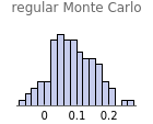
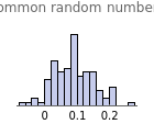
The Demonstration output shows that is a modestly better way to estimate - than -. The histogram on the left features a simulated collection of the quantity -. The histogram on the right features a simulated collection of the quantity .
M
3
μ
1
μ
2
M
1
M
2
M
1
M
2
M
3
Run the simulation repeatedly to see that in this example, the method of common random numbers always results in a reduction of variance.