The Arnold Problem
The Arnold Problem


Consider the unsteady-state evaporation of a liquid, the Arnold problem. The governing equation is:
∂c
∂t
2
∂
∂
2
z
D
1-
c
A0
∂c
∂z
z=0
∂c
∂z
where is the diffusion coefficient.
D
The initial and boundary conditions are:
t=0
c(z,0)=0
z=0
c(0,t)=
c
A0
z=∞
c(∞,t)=0
where is the interfacial gas-phase concentration and is the position.
c
A0
z
This equation has an analytical solution:
c(z,t)/=
c
A0
1-erf(Z-ϕ)
1+erf(ϕ)
Z=
z
4Dt
ϕ
ϕ=
1
π
c
A0
(1-)
c
A0
-
2
ϕ
e
(1+erf(ϕ)
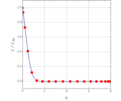
This Demonstration plots the solution . The numerical solution obtained using Chebyshev orthogonal collocation is given by the red dots. The analytical solution is given by the blue curve. Excellent agreement between both solutions is observed. You can vary the values of , , and as well as the number of Chebyshev collocation points, .
c(z,t)
t
D
c
A0
N+1