Radioactive Decay in the Causal Interpretation of Quantum Theory
Radioactive Decay in the Causal Interpretation of Quantum Theory


According to classical physics, a particle can never overcome a potential greater than its kinetic energy; this is not the case in quantum theory. For unstable isotopes there is a finite probability for a quantum particle (an particle) to tunnel through the potential barrier in a nucleus. Such isotopes are called radioactive isotopes. The behavior of such isotopes can be described by a square wave packet that is a solution of the Schrödinger equation with the potential term . The time evolution leads to a wave packet that bounces back and forth. Each time it strikes the potential barrier a part of the packet tunnels through and there is a chance for some transmission. In orthodox quantum theory it is impossible to predict the decay of a single isotope. A statistical conclusion can be made only for an ensemble of isotopes (e.g., half-life period).
α
V
In the causal interpretation of quantum theory of David Bohm, it is in principle possible to predict the decay of a single isotope (single event). Radioactive decay is described deterministically in terms of well-defined particle trajectories. In practise, it is impossible to predict or control the quantum trajectories with complete precision. Single particles are placed in a wave packet inside a nuclear potential. The decay of an isotope only depends on the initial position of the particle inside the wave packet. If the position is at the front of the wave, the particle trajectory leads to an escape of the particle from the nucleus. In the region of the potential, the quantum potential becomes large, and the resulting particle acceleration together with the reduction of the nuclear potential via the quantum potential accounts for tunneling.
α
For this Demonstration a simple model of radioactive decay is chosen. The nuclear potential is proportional to (Pöschl–Teller potential) with the potential height . The initial unnormalized wave is =, with (width of the initial wavefunction) and (wave number). The peak is placed at =0.3. The initial positions of the particles are linearly distributed around the peak of the packet inside the wave. If , the packet evolves like a free packet. For , none of the particles inside the wave packet leave the nuclear potential (stable isotope).
V
potH
2
sech(ax+X)
potH
ψ
0
-2
2
(x+)
x
0
2
ρ
e
ikx
e
ρ=0.06
k=120
x
0
potH=1
potH=8001
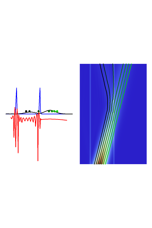
The trajectories are positioned in space. The graphic on the left shows the particles' positions, the wavefunction amplitude (black), the Pöschl–Teller potential (blue), and the quantum potential (red). The graphic on the right shows the amplitude of the wavefunction, the potential for the complete time period, and the trajectories at the actual time step. The wavefunction amplitude, the potential, and the quantum potential are scaled to fit.
(x,t)
R
R