Pulsatile Flow in a Circular Tube
Pulsatile Flow in a Circular Tube


The velocity distribution, , is computed numerically using NDSolve for a pulsatile pressure-driven flow in a tube. This model considerably simplifies the actual flow through veins and arteries.
u(r,t)
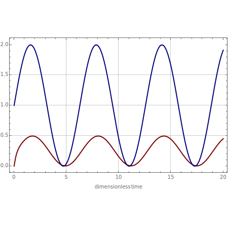
When the kinematic viscosity is large and momentum diffusion is fast (i.e. the Strouhal number, , is small, as shown in the first snapshot), the velocity at the center of the tube, (shown in red), can instantaneously adjust to changing pressure, (shown in blue). The velocity is then in phase with the pressure gradient.
R
w
u(r,t)
-(t)
∂p
∂z
On the other hand, when the kinematic viscosity is small and momentum diffusion is slow, then is large (see the second snapshot) and the velocity at the center of the tube, , lags the pressure gradient by 90°.
R
w
u(r,t)
The long-time analytical solution (given in Details and shown in green on the plot for =1) matches the numerical solution very well, after a short transient period. This derivation can be found in [1–2].
R
w
One can see that when everything is in phase then the flow behaves locally as a quasi-steady Poisueille flow, in which the green and blue curves coincide, the green curve being the parabolic solution and the blue curve taking inertial effects into account. At a high Strouhal number, inertial effects become significant and the velocity field is no longer locally parabolic (green and blue curves are distinct). Both limiting cases are shown in the last two snapshots.