Particle Position Distribution Using a Brownian Dynamic Simulation
Particle Position Distribution Using a Brownian Dynamic Simulation


The Brownian dynamics (BD) method is used to solve two case studies for the position distribution of a particle in: (1) a flowing fluid under no external force and Brownian diffusion; and (2) a quadratic energy well with Brownian diffusion. For both cases, the explicit Euler stochastic differential equation (SDE) method is employed [1].
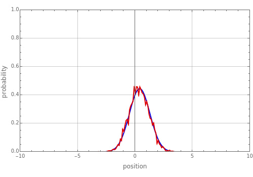
First, the Demonstration computes the probability distribution function at time for a particle in fluid flow with no external force. The BD simulation result, shown in red, is in agreement with the solution of the convection/diffusion equation, shown in blue and given by , where is the fluid flow velocity, , and is the diffusion coefficient. The values of the fluid flow velocity and diffusion coefficient can be modified. When the diffusion coefficient is small, the distribution curve is narrow. For high positive (negative) fluid flow velocities, the peak shifts to the right (left).
t=0.2
f(x,t)=exp(σ
-
2
(x-Vt)
2
2
σ
2π
)V
σ=
2Dt
D
Secondly, the Brownian dynamics technique is used to determine the position distribution for a spherical particle in a quadratic energy well, . The BD result shown in red agrees with the theoretical distribution shown in blue. You can vary the values of the spring constant, , as well as the diffusivity, . Increasing the spring constant or decreasing the diffusivity leads to narrower distributions.
U(x)=k/2
2
x
k
D