Nonparametric Regression and Kernel Smoothing: Confidence Regions for the L2-Optimal Curve Estimate
Nonparametric Regression and Kernel Smoothing: Confidence Regions for the L2-Optimal Curve Estimate

This Demonstration considers one of the simplest nonparametric-regression problems: how to "optimally denoise" a noisy signal, assuming it is a smooth curve plus a realization of i.i.d. centered Gaussian variables of known variance . The setting is the same as in the Demonstration "Nonparametric Curve Estimation by Kernel Smoothers: Efficiency of Unbiased Risk Estimate and GCV Selectors". Recall that applying a classical kernel-smoothing method to a noisy signal actually produces a trajectory of candidate estimates of the underlying curve, each estimate being associated with (or tuned by) a bandwidth value, denoted . Ideally one would like to pick "the optimal " given the data. A classical approach is to attempt (as in the previously mentioned Demonstration) to minimize over the average of the squared errors , which is a discrete version of the distance between the underlying (true) curve and the curve estimate obtained with (see Details). The unknown true minimizer (resp. the associated curve estimate) is called the ASE-optimal bandwidth (resp. the -optimal curve estimate).
2
σ
h
h
h
ASE(h)
L
2
h
L
2
This Demonstration implements a simulation-based method, proposed in [1], for constructing approximate confidence intervals for the ASE-optimal bandwidth, and shows why Mathematica's built-in Manipulate function is especially appropriate to inferences that are made possible by such intervals (e.g. to give an answer to the question, "Is the -optimal curve estimate rather accurately located with a confidence of, say, 90%?").
L
2
The data processing in this program assumes that is known, so the criterion (unbiased estimate of ) is then available in place of GCV. This restriction is for simplicity because the augmented-randomization would otherwise require an estimate of and a number of quite different methods are available for such an estimate.
σ
C
L
ASE(h)+
2
σ
2
σ
For a given percentile number , chosen between 1 and 50, such a construction consists of:1. simulating a large number (here 1000) of randomized- criteria (to be more precise, each criterion uses a randomized-trace function with "augmented randomness" as defined in [1], and is referred to as an ARCL criterion),2. minimizing each of these 1000 criteria, and3. taking the and percentiles of the population of the 1000 minimizers.
p
C
L
th
p
th
(100-p)
It is shown in [1] that the percentiles of the population that could be obtained in theory at step 2 if the number of simulations (here 1000) were increased to infinity, yields asymptotically (i.e. as the size of the dataset tends to infinity) conservative statements.
Precisely, assuming that the asymptotic regime is attained, the (respectively ) percentile will be less (resp. greater) than the ASE-optimal bandwidth with a probability at least . This last probability is thus the so-called nominal coverage probability, denoted by or . Notice that we only consider the case of an identical nominal coverage for the lower bound and the upper bound (equal-tail interval). The (asymptotically guaranteed) coverage of the two-sided interval is thus .
th
p
th
(100-p)
1-p/100
C(lower)
C(upper)
1-p/50
In this Demonstration, if is chosen between 50 and 99, then plays the role of in the previous paragraph.
p
100-p
p
The true curve can be chosen among six possible choices and the size of every simulated set of data is fixed at 1024 (although this can be modified in the program). You can vary the "noise level" from a relatively small level (with respect to the "magnitude" of the true curve, here about 1) to a rather large one. You can select the checkbox "include data in the plot".
σ
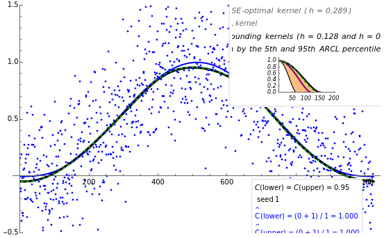
You can fix by choosing for it to be among typical percentile values, say 95 (and or are thus fixed at 0.95), and clicking the tab with label ARCL percentile curve estimate ...". You can then see the first view of the results (detailed below) obtained when analyzing the dataset generated with seed set to 1.
p
C(lower)
C(upper)
"
th
95
Now, clicking the "Play" button for the slider "seed for data generation" repeats, for a succession of simulated datasets, the following three tasks:
• first the confidence interval for the ASE-optimal bandwidth is constructed (steps 1, 2, and 3 above run rather quickly in this program thanks a Fourier domain implementation and some precomputation);
• next the two "bounding kernels at level %", corresponding to the lower and upper limits of the confidence interval, are plotted in black in the additional panel, top right of the view 1 (also plotted in the main panel, in black, is the ARCL-percentile curve estimate; that is the one with bandwidth equal to the percentile of the 1000 bandwidths obtained in step 3 above);
p
th
p
th
p
• and the two empirical coverages are updated by simply checking for the current dataset whether or not the ASE-optimal kernel (plotted in dashed green) is really bounded by the above bounding kernels.
After having automatically processed, say, a few hundred datasets that differ only by their seed, this can first demonstrate that the constructed confidence regions are often very good (see the Details below): indeed, we have experienced that in the few cases when such a region is not conservative, the empirical coverage converges (as more and more seeds are processed) to a value lower than the nominal probability, but only by a small amount.
In addition, the animation so obtained in the first view by clicking the "Play" button also allows an assessment of the variability of the two bounding kernels.
Next, and perhaps more importantly, by clicking the "Pause" button, selecting the second view, and moving the slider "trial bandwidth ", you can observe that a "large" difference between the lower bound and the upper bound (with a coverage probability fixed at, say, 0.90) for the ASE-optimal bandwidth, does not necessarily imply a large difference between the corresponding curves that delimit the confidence region (curves in orange) for the ASE-optimal curve estimate (see Details).
h
T
The way the two coverages are updated is coded similarly to the Demonstration "How Do Confidence Intervals Work?", except that the statement (viz. the constructed "bounding" bandwidth is a true bound) is with respect to an unknown "parameter" (the ASE-optimal bandwidth) that varies here from seed to seed, whereas it is a constant (like the usual "mean value") in that Demonstration.