Kolmogorov Complexity of 3×3 and 4×4 Squares
Kolmogorov Complexity of 3×3 and 4×4 Squares


Which of "11111111111111111111", "15747363020045852837", or "81162315385411264758" can be described in the most compact way? Each can be described as it is presented, using 20 characters. The first two could be described by and . The Kolmogorov complexity measures the length of the shortest program required to reproduce a pattern.
((-1)9)
20
10
⌊(π+e)^25⌋
K
This Demonstration provides Kolmogorov complexity approximations to 3×3 and 4×4 square arrays. The approximations come from applying the Levin–Chaitin algorithmic coding theorem that relates the frequency of the appearance of a pattern and its Kolmogorov complexity. The coding theorem method [3, 4] consists, for this Demonstration, in the calculation of the output frequency distribution of Turing machines with five states and two symbols operating on a two-dimensional grid (instead of the traditional one-dimensional tape).
1.291×
12
10
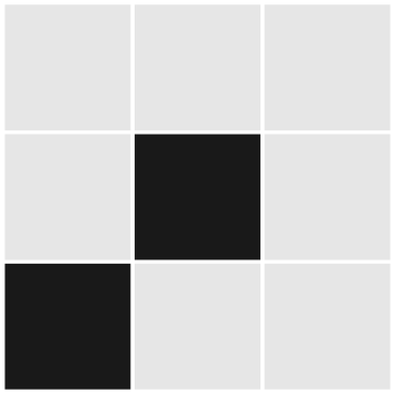
According to the coding theorem, the Kolmogorov complexity of a pattern is , where is the frequency of occurrence of ; this non-integer Kolmogorov complexity is denoted by [1]. You can either select a pattern using the bar or click directly on the squares of the grid for a desired configuration. The Demonstration will then display the Kolmogorov complexity value for the chosen grid.
s
K(s)=-m(s)
log
2
m(s)
s
K
m
The Compress function in Mathematica is another, more traditional way to approximate Kolmogorov complexity, and is shown for comparison, but unlike the coding theorem, lossless compression techniques do not deal well with small patterns.