k-Nearest Neighbor (kNN) Classifier
k-Nearest Neighbor (kNN) Classifier


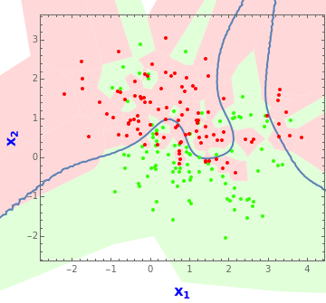
In a typical classification problem we wish to predict the output class, , given inputs, and . In the prototypical problem illustrated above, the observed training data consists of observations equally divided between the two classes. The 0/1 values are color-coded green and red. Based on this training data, our object is to find a predictor for new data, designated the test data. One method is to take the nearest neighbors of the new inputs and predict the new output based on the most frequent outcome, 0 or 1, among these neighbors. By taking odd we avoid ties. This is the kNN classifier and the idea is easily generalized to more than two output classes and more than two inputs. The kNN classifier is one of the most robust and useful classifiers and is often used to provide a benchmark to more complex classifiers such as artificial neural nets and support vector machines.
y∈{0,1}
p=2
x
1
x
2
n=200
k
k
In this simple example, Voronoi tessellations can be used to visualize the performance of the kNN classifier. The solid thick black curve shows the Bayes optimal decision boundary and the red and green regions show the kNN classifier for selected .
k
Based only on this training dataset, it can be shown that is the best possible choice for . With , the expected misclassification rate on future data is minimized. See below for details.
k=17
k
k=17
In practice, though, we need to base the choice of solely on the training dataset. The pseudo-likelihood method of Holmes and Adams (2003) produces =7 while leave-one-out cross-validation yields =3. Linear or logistic regression with an intercept term produces a linear decision boundary and corresponds to choosing kNN with about three effective parameters or .
k
k
k
k≐67