Estimating a Centered Matérn (1) Process: Three Alternatives to Maximum Likelihood via Conjugate Gradient Linear Solvers
Estimating a Centered Matérn (1) Process: Three Alternatives to Maximum Likelihood via Conjugate Gradient Linear Solvers


The setting is the same as in the Demonstration "Three Alternatives to the Likelihood Maximization for Estimating a Centered Matérn (3/2) Process", except that the "differentiability" parameter (often denoted by ) is fixed here to 1. This value 1 for is classically used in two dimensions following the seminal work of Whittle [1]. The corresponding autocorrelation function has the simple expression (the process variance being denoted by ), where (·) is a modified Bessel function of the second kind (see the Details section in the help page for the BesselK function) and is still called the inverse-range parameter, being the "range" (or "support") of .
ν
ν
ρ(t,θ)==(θt)(θt)
[x(s+t)x(s)]
2
τ
K
1
2
x(s)
2
τ
K
1
θ>0
-1
θ
ρ(·,θ)
One important difference with the case is that the considered process, even regularly sampled (here observed at in the set ), no longer coincides with any ARMA time series. Fast Fourier transforms (FFT) are then invoked for the simulation of such a series.
ν=3/2
t
{0,δ,2δ,…,(n-2)δ,(n-1)δ=1}
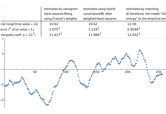
The same three methods as in the case are implemented here for estimating and , namely: Cressie's weighted least-squares method [4], the "hybrid" Zhang–Zimmerman method [5], and the recently proposed "CGEM-EV" method [6], here in the case of no measurement error. For each of the three methods, the estimate of the so-called "microergodic coefficient", which is now (the general expression for being ), is naturally defined as the square of the product of the estimates of and .
ν=3/2
τ
θ
c=
2
τ
2
θ
c
c=
2
τ
2ν
θ
τ
θ
For all the simulated time series, the true variance is fixed to 1 (this choice is without loss of generality), and various can be tried for the true value of the inverse-range parameter. The legends for the table of the numerical results are similar to the ones in the above-mentioned Demonstration for the case .
2
τ
θ
ν=3/2
Let denote the candidate correlation matrix of , with inverse-range , that is, the matrix whose element in the row and column is =ρ(i-jδ,θ). The only difficulty regarding implementation in the case of no measurement error, of both the hybrid method and CGEM-EV, is the computation of the quadratic form x,x, the so-called "Gibbs energy of associated with a given ".
R(θ)
x={x(0),x(δ),…,x((n-2)δ),x(1)}
θ
n×n
th
i
th
j
[R(θ)]
i,j
1
n
-1
R(θ)
x
θ
The computation of x uses a conjugate-gradient (CG) solver preconditioned by a classical factored sparse approximate inverse (FSAI) preconditioning (see [7] for a recent survey), each product by being obtained via FFT from the standard embedding of in a circulant matrix.
-1
R(θ)
R(θ)
R(θ)
2n×2n
It is important to notice that becomes ill-conditioned for large and decreasing toward the lower-bound used here (as in the Demonstration for ); so using a preconditioner is a mandatory requirement to accelerate the CG convergence.
R(θ)
n
θ
θ=1.5
ν=3/2
It is observed here that this implementation is quite fast, even for .
n=8196