Energies for Particle in a Gaussian Potential Well
Energies for Particle in a Gaussian Potential Well


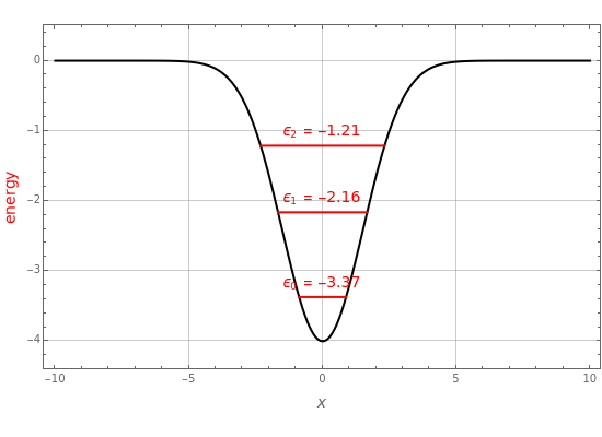
The Schrödinger equation for a particle in a one-dimensional Gaussian potential well , given by , has never been solved analytically. This Demonstration derives an approximation for the first few bound-state energies, <0, using the linear variational method. The wavefunction is approximated by a linear combination . It is convenient to take the basis functions (x) as the corresponding orthonormalized eigenfunction of the linear harmonic oscillator: (x)=n!(, where is the Hermite polynomial and is a scaling constant to be determined variationally. After evaluating the matrix elements =(x)-+V(x)(x)dxover the selected set of basis functions, Mathematica can calculate the eigenvalues in a single step, from which we select only those with negative values. For convenience, we set , so that all distances are expressed in bohrs (Bohr radii) and energy quantities in hartrees.
V(x)=-
V
0
-2
2
x
2
σ
e
-ψ''+V(x)ψ(x)=ϵψ(x)
2
ℏ
2m
(x)
ϵ
n
ψ(x)=(x)
N-1
∑
n=0
c
n
ϕ
n
ϕ
n
ϕ
n
1
n
2
1/4
α
π
-α2
2
x
e
H
n
α
x)H
n
th
n
α
H
nm
∞
∫
-∞
ϕ
n
1
2
2
d
d
2
x
ϕ
m
N
N
ℏ=m=1
The graphic shows the computed energy levels for selected values of , , , and , superposed on the potential energy function. By an estimation based on the WKB method, the number of bound states is approximated by .
V
0
σ
α
N
floor4σ+
V
0
2π
1
2
The approximate eigenfunctions (x) can also be calculated, applying the the built-in Mathematica function Eigenvectors. Since the resulting functions have very similar shapes and nodal structures as the corresponding harmonic oscillator eigenfunctions, we did not consider it worthwhile to include these in the Demonstration.
ψ
n