Concentration Distributions with a Position-Dependent Diffusion Coefficient
Concentration Distributions with a Position-Dependent Diffusion Coefficient


This Demonstration shows plots of the steady-state concentration distribution through a plane sheet, a cylindrical annulus, and a spherical shell, in which diffusion is assumed to be one-dimensional. Different values of parameter can be chosen.
α
The relevant equations are:
For the plane sheet, D=0 for , where is the diffusion coefficient. Without loss of generality, one can choose the boundary conditions and .
∂
∂x
∂c
∂x
0⩽x⩽1
D=1+αx
c(x=0)=1
c(x=1)=0
For the cylindrical annulus, Dr=0 for =1⩽r⩽=2, where is the diffusion coefficient. Again, one can choose the boundary conditions and .
1
r
∂
∂r
∂c
∂r
r
1
r
2
D=1+αr
c(r=1)=1
c(r=2)=0
For the spherical shell, D=0 for =1⩽r⩽=2, with the same and boundary conditions as for the cylindrical annulus.
1
2
r
∂
∂r
2
r
∂c
∂r
r
1
r
2
D
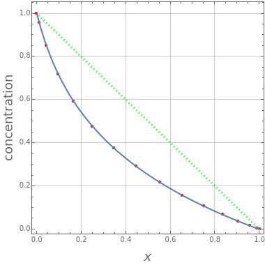
For the plane sheet, if , then is a constant and the concentration distribution is indicated by the dotted green line. Fick's second law is recovered, as shown in the first snapshot.
α=0
D=1
In all plots, the red dots correspond to the solution obtained using Chebyshev orthogonal collocation with collocation points. The blue curve is the analytical solution given by Crank [1]: , where with =0 (planar case) and =1 (cylindrical and spherical cases).
N=16
1-c=-I-
I
1
I
1
I
2
I(x)=(1+αξ)dξ
x
∫
x
0
1
m
ξ
x
0
x
0
For the plane sheet, , =I(x=0)=0, and =I(x=1).
m=0
I
1
I
2
For the cylindrical annulus, , =I(r=1)=0, and =I(r=2).
m=1
I
1
I
2
For the spherical shell, , =I(r=1)=0, and =I(r=2).
m=2
I
1
I
2
As expected, the two solutions agree perfectly.