Chaotic Data: Maximal Lyapunov Exponent
Chaotic Data: Maximal Lyapunov Exponent


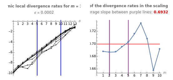
This Demonstration obtains estimates of the maximal Lyapunov exponent for four chaotic datasets (each of length 4000). The data is derived from the logistic, Hénon and Lorenz models and NMR laser data. The figure on the left displays logarithmic divergence rates for some embedding dimensions (as functions of a time distance ). They are calculated at discrete points, which are joined with lines. The logarithmic divergence rates, which require significant computation times, were calculated outside of this Demonstration (for these computations, see "Analysis of Chaotic Data with Mathematica" in the Related Links).
m
δ
We first search for a so-called scaling region where the divergence rates develop approximately linearly with very similar slopes for several values of . This is represented by the two blue vertical lines. A linear fit for the divergence rates between the vertical lines (endpoints included) is then computed for each . The slopes of these lines are shown in the right-hand plot for each value of . If, for some scaling region, we get slopes that are approximately constant for several values of , this constant is an estimate of the maximal Lyapunov exponent. We denote the region of these slopes with the two purple vertical lines. The figure then shows the average slope between these lines (endpoints included); this average is an estimate of the maximal Lyapunov exponent. The red line can be used to check the constancy of the selected slopes. The first figure also shows the interval between neighboring data points.
m
m
m
m
ϵ