Brauer's Cassini Ovals versus Gershgorin Circles
Brauer's Cassini Ovals versus Gershgorin Circles


This Demonstration gives different views of the neighborhood of the spectrum of a matrix acting in , with low dimension . It continues the ideas presented in the Demonstration "Enclosing the Spectrum by Gershgorin-Type Sets", offering extensions that go by the names of Brauer, Ostrowski, and others.
A
n
n
We are looking for the eigenvalues of ; we can offer some easily derivable ensembles of sets covering their location, consisting of members with a simple description and low computational cost.
A
To illustrate the ideas, a family of random complex matrices with dimensions from 2 to 15 is selected. You can choose whether the matrix is normal, diagonalizable, or deficient, each being built from (almost) the same spectrum.
First, to get an impression of the area in the complex plane where the matrix "lives", the location of the points, the hub, the convex hull, and its boundary fence can be shown, independently for all the entries of , for its diagonal entries, and for its eigenvalues.
A
A
What we call the "hub" of is the mean of the diagonal entries of , which is at the same time the mean of the eigenvalues of . In the literature this is usually expressed as tr(A), an invariant under similarity. We call it the hub of because, for all matrices similar to , it represents the center of gravity of their respective diagonal entries, which is common to them all, as well as the center of gravity of their common spectrum, so it is the natural pivot point for the whole similarity class of . Indeed, one could claim that the whole question of similarity of a matrix hinges on this point! Here it is marked as a yellow point with a red boundary.
A
A
A
1
n
A
A
A
A
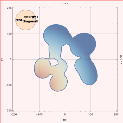
The total energy of a matrix is defined as , its distribution between the diagonal and rest of the matrix can be popped up, too. For normal matrices the total energy is an invariant under unitary similarity, its distribution between diagonal and rest depends on how close the diagonal of approximates the spectrum. For non-normal matrices the total energy does not need to be constant within a similarity class.
A
tr(A)
*
A
A
A
In addition, you can experiment with a unitarily similarized version of via a parameter between 0 and 1, showing a possible passage from to its Schur similarity , thereby resembling a Jacobi tour. For every , has the same eigenvalues as , and carries them on its diagonal.
A
Sim
A
κ
A
A
Schur
κ
A
Sim
A
A
Schur
The ideas of Gershgorin, Brauer, Ostrowski, and others can be made explicit with the help of the next block of controls. Get familiar with some of their contributions and compare their respective benefits or drawbacks!
If you would like to focus your attention on even simpler regions, such as a single disk or a circular ring, you can find some circles that enclose or exclude the whole or parts of the spectrum of . Their centers might be chosen as the mean of the points (i.e. the hub), as the center of area of the convex hull, or as the "best" center with the smallest radius.
A
Last but not least, the "numerical range frame" gives a cover of the spectrum by a simple rectangle, at the expense of having to calculate four eigenvalues, two of the Hermitian part of and two of the skew-Hermitian part of .
A
A
To familiarize yourself with what is shown, start with the settings of a snapshot. Almost every item in the graphics is annotated, so mouseover the graphics to see explanations and click buttons one after the other. After any change, mouseover the graphic again. Although almost every item is explained, some annotations only show up when the respective items are not shadowed by other ones. Resize the graphics area. Look at the impact of loading the diagonal by using the "" slider. Look at the impact of changing the matrix type. Switch between Gershgorin and Brauer methods and between sum and Euclid norms. Look at the relation between the convex hull of the eigenvalues and the numerical range frame, especially for different matrix types.
4
κ