Wolfram Cloud Document

Evaluate

Acceleration of Particles in a Wave Obeying the Korteweg-de Vries Equation

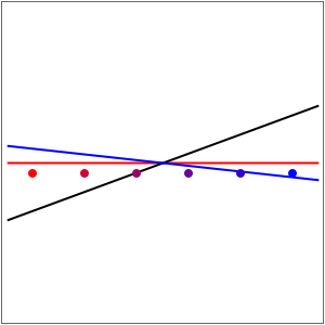
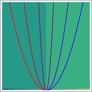
Manipulate

KdV[i,choice,ImageSize{300,300}],{{i,50,"time steps"},1,50,1,Appearance"Labeled",ImageSizeTiny},

Delimiter,

{{choice,1,"function choice"},{1,2},ControlType"RadioButton"},

ControlPlacementTop,

SaveDefinitionsTrue,

InitializationKdV[i_,choice_,opts___]:=QuietModule{tStart,tEnd,xR,xL,xP,dt,intervall,dpAll,pathAll,

points,colors,vPlot,qPlot,aPlot,uPlot,para},

para=p

;

tStart=0;

tEnd=5;

xR=16;

xL=-16;

u[x_,t_]=6x/(1+36t),

Sech

t-px)

/.para;

v[x_,t_]=

18x

1+36t

/.para;

a[x_,t_]=-

324x

(1+36t)

,0;

qp[x_,t_]=0,p

-1+

1+Cosh[p

t-px]

/.para;

xP=0;

sol=DSolve[{x'[t]v[x[t],t][[choice]],x[0]x0},x[t],t]//Flatten;

Print"Proof that acceleration is equal to a=

FractionBox[\(∂\), \(∂x\)](FractionBox[\(\*SubscriptBox[\(∂\),

\(xx\)]\u\), \(u\)]+3uSuperscriptBox[\()\), \(2\)]:"

D[x[t]/.sol[[1]],t,t]==-

∂



∂

x,x

u[x,t][[choice]]

+3u[x,t][[choice]]^2/.x->x[t]/.sol[[1]]//FullSimplify

xAnalytic[t_]:=Tablex[t]/.sol[[1]]/.x0xP+dx,dx,-

;

xPosition[t_,l1_Integer]:=xAnalytic[t][[l1]];

intervall=50;

dt=(tEnd-tStart)/(intervall);

colors=Table[Blend[{Red,Blue},x],{x,0,1,0.2}];

dpAll=ContourPlot[u[x,t][[choice]],{x,xL,xR},{t,tStart,tEnd},MeshFalse,PlotRangeAll,ColorFunction

"BlueGreenYellow",ContourStyleNone,PerformanceGoal"Quality",MaxRecursionControlActive[0,

Automatic],PlotPointsControlActive[40,50]];

pathAll=Table[ParametricPlot[{xPosition[t,l1],t},{t,tStart,idt+tStart},PlotStyle{colors[[l1]],Thick},

PerformanceGoal"Speed"],{l1,1,Length[xAnalytic[t]],1}];

points=Table[Graphics[{AbsolutePointSize[8],colors[[j]],Point[{xPosition[t,j]/.t(tStart+dti),-0.1}//

Flatten]}],{j,1,Length[xAnalytic[t]]}];

vPlot=PlotEvaluate

v[x,tStart+dti][[choice]],{x,xL,xR},PlotRange{-1.5,1.5},PlotStyle{Green,

Thick},PerformanceGoal"Speed";

qPlot=Plot[Evaluate[qp[x,tStart+dti]][[choice]],{x,xL,xR},PlotRange{-1.5,1.5},PlotStyle{Red,Thick},

PerformanceGoal"Speed"];

aPlot=Plot[Evaluate[a[x,tStart+dti]][[choice]],{x,xL,xR},PlotRange{-1.5,1.5},PlotStyle{Blue,Thick},

PerformanceGoal"Speed"];

uPlot=Plot[u[x,tStart+dti][[choice]],{x,xL,xR},PlotRange{-1.5,1.5},PlotStyle{Black,Thick},

PerformanceGoal"Speed"];

Grid[{{

Show[{(*vPlot,*)qPlot,uPlot,aPlot,points},opts,AxesFalse,AspectRatio2/2,FrameTicksNone,

FrameTrue,BackgroundWhite],

Show[{dpAll,pathAll},opts,AxesFalse,AspectRatio2/2,FrameTicksNone,FrameTrue,PlotRangeAll]

}}]



time steps

function choice