Data and Design Matrix
y={3,1,2,2,1,3,2,13,14,15,18,16,13,17,12,13};DM={{1,0},{1,0},{1,0},{1,0},{1,0},{1,1},{1,1},{1,1},{1,1},{1,1},{1,1},{1,1},{1,1},{1,1},{1,1},{1,1}};DM=Map[{#1[[1]],If[#1[[2]]1,0,1]}&,DM]
{{1,1},{1,1},{1,1},{1,1},{1,1},{1,0},{1,0},{1,0},{1,0},{1,0},{1,0},{1,0},{1,0},{1,0},{1,0},{1,0}}
Run the (Poisson) GLM and get the parameter table
poi=GeneralizedLinearModelFit[{DM,y},ExponentialFamily"Poisson"];poi["ParameterTable"]
Estimate | Standard Error | z-Statistic | P-Value | |
#1 | 2.51476 | 0.0857486 | 29.3271 | 4.68008× -189 10 |
#2 | -1.92697 | 0.344185 | -5.59866 | 2.16018× -8 10 |
Function that calculates the likelihood of the Poisson GLM
ll[b0_,b1_,y_]:=Module[{lp=Exp[DM.{b0,b1}]},Inner[PDF[PoissonDistribution[#1],#2]&,lp,y,Times]]
Find Maximum using optimization
maxsol=NMaximize[ll[b0,b1,y],{b0,b1}]
{3.97312×,{b02.51476,b1-1.92697}}
-20
10
Compute the Hessian & the observed Fisher information matrix
Hess=D[Log[ll[b0,b1,y]],{{b0,b1},2}];
Sqrt[-Inverse[Hess/.{b0maxsol[[2,1,2]],b1maxsol[[2,2,2]]}]]
{{0.0857493,0.+0.0857493},{0.+0.0857493,0.344186}}
Bayesian Normalization Constant
Z=NIntegrate[ll[b0,b1,y]/ll[poi["ParameterTableEntries"][[1,1]],poi["ParameterTableEntries"][[2,1]],y],{b0,-Infinity,Infinity},{b1,-Infinity,Infinity},Method->"GaussKronrodRule"]
0.181374
Multivariate Normal Approximation Normalization Constant
Sqrt[Det[poi["CovarianceMatrix"]]]*2*Pi
0.179591
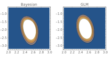
Plot the Bayesian and the Multivariate Normal (Frequentist) Densities For the Parameters
Plot3D[{ll[b0,b1,y]/ll[poi["ParameterTableEntries"][[1,1]],poi["ParameterTableEntries"][[2,1]],y]/Z,PDF[MultinormalDistribution[poi["BestFitParameters"],poi["CovarianceMatrix"]],{b0,b1}]},{b0,2.,3},{b1,-3.2,-0.6},PlotRangeAll,PlotLegends{"Bayesian","GLM"},PerformanceGoal"Quality",PlotPoints50]

Show results as Contour Plots
Show[GraphicsRow[{ContourPlot[ll[b0,b1,y]/ll[poi["ParameterTableEntries"][[1,1]],poi["ParameterTableEntries"][[2,1]],y]/Z,{b0,2.,3},{b1,-3.2,-0.6},PlotLabel"Bayesian",AxesLabel{B0,B1}],ContourPlot[PDF[MultinormalDistribution[poi["BestFitParameters"],poi["CovarianceMatrix"]],{b0,b1}],{b0,2.,3},{b1,-3.2,-0.6},PlotLabel"GLM",AxesLabel{B0,B1}]}]]
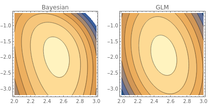
Plot the Bayesian and the Multivariate Normal (Frequentist) Log Densities For the Parameters
Plot3D[{Log[10,ll[b0,b1,y]]-Log[10,ll[poi["ParameterTableEntries"][[1,1]],poi["ParameterTableEntries"][[2,1]],y]]-Log[10,Z],Log[10,PDF[MultinormalDistribution[poi["BestFitParameters"],poi["CovarianceMatrix"]],{b0,b1}]]},{b0,2.,3},{b1,-3.2,-0.6},PlotRangeAll,PlotLegends{"Bayesian","GLM"},PerformanceGoal"Quality",PlotPoints50]

Show results as Contour Plots for the log - density
Show[GraphicsRow[{ContourPlot[Log[10,ll[b0,b1,y]]-Log[10,ll[poi["ParameterTableEntries"][[1,1]],poi["ParameterTableEntries"][[2,1]],y]]-Log[10,Z],{b0,2.,3},{b1,-3.2,-0.6},PlotLabel"Bayesian",AxesLabel{B0,B1}],ContourPlot[Log[10,PDF[MultinormalDistribution[poi["BestFitParameters"],poi["CovarianceMatrix"]],{b0,b1}]],{b0,2.,3},{b1,-3.2,-0.6},PlotLabel"GLM",AxesLabel{B0,B1}]}]]
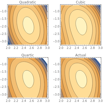
Is the quadratic approximation to the likelihood accurate?
Are the differences between Bayesian and frequentist solutions due to higher order properties of the log-Likelihood that are discarded in the conventional frequentist treatment, rather than the Bayesian approach itself?
Are the differences between Bayesian and frequentist solutions due to higher order properties of the log-Likelihood that are discarded in the conventional frequentist treatment, rather than the Bayesian approach itself?
quadLL[B0_,B1_,b0_,b1_,y_]:=Normal[Series[Log[10,ll[(B0-b0)*t+b0,(B1-b1)*t+b1,y]],{t,0,2}]]/.{t1};cubLL[B0_,B1_,b0_,b1_,y_]:=Normal[Series[Log[10,ll[(B0-b0)*t+b0,(B1-b1)*t+b1,y]],{t,0,3}]]/.{t1};quartLL[B0_,B1_,b0_,b1_,y_]:=Normal[Series[Log[10,ll[(B0-b0)*t+b0,(B1-b1)*t+b1,y]],{t,0,4}]]/.{t1};
Show[GraphicsGrid[{{ContourPlot[quadLL[B0,B1,poi["ParameterTableEntries"][[1,1]],poi["ParameterTableEntries"][[2,1]],y],{B0,2.,3},{B1,-3.2,-0.6},PlotLabel"Quadratic"],ContourPlot[cubLL[B0,B1,poi["ParameterTableEntries"][[1,1]],poi["ParameterTableEntries"][[2,1]],y],{B0,2.,3},{B1,-3.2,-0.6},PlotLabel"Cubic"]},{ContourPlot[quartLL[B0,B1,poi["ParameterTableEntries"][[1,1]],poi["ParameterTableEntries"][[2,1]],y],{B0,2.,3},{B1,-3.2,-0.6},PlotLabel"Quartic"],ContourPlot[Log[10,ll[B0,B1,y]],{B0,2.,3},{B1,-3.2,-0.6},PlotLabel"Actual"]}}]]