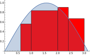
Riemann Sum

Approximating the definite integral.
June 22, 2017—Itzel Carolina Delgadillo Perez

Explanation

Let’s suppose you want to obtain the area under the curve in a plot.
Example curve and area:
In[]:=
area=NIntegrate[Sin[x],{x,0,Pi}];​​Grid[{​​{functionPlot:=Plot[Sin[x],{x,0,Pi},FillingAxis,ImageSizeMedium];functionPlot},​​{"Actual area: "<>ToString[area//N]}​​}]
Out[]=
Actual area: 2.
If you were drawing the curve on paper, it’s not really possible to measure it directly as it is. The most naive approach is to draw geometrical figures for which is known how to calculate their areas—for example, rectangles.
Represent the curve as rectangles:
In[]:=
rectCoord={​​{{0.5,0},{Pi-0.5,0},{Pi-0.5,Sin[0.5]},{0.5,Sin[0.5]}},​​{{1.0,Sin[0.5]},{Pi-1,Sin[0.5]},{Pi-1,Sin[1]},{1,Sin[1]}}​​};​​bars=Map[Graphics[​​ EdgeForm[{Thickness[Medium],Black}],​​ Red,​​ Polygon[#]​​]&,​​rectCoord​​];​​rectArea=Plus@@Map[Area@Polygon[#]&,rectCoord];​​error:=Abs[area-rectArea];​​Grid[{​​{Show[Flatten[{functionPlot,bars,functionPlot}],ImageSize->Medium]},​​{"Rectangle area "<>ToString[rectArea//N]},​​{"Actual area "<>ToString[area//N]},​​{"Error "<>ToString[error//N]}​​}]
Out[]=
Rectangle area 1.44004
Actual area 2.
Error 0.559957
We can simplify our approximation by making the rectangles’ heights dependent on the curve’s values. For example:
Now the rectangle height depends on the curve height:
In[]:=
rectXCoord=​​ {0,0.6},​​ {0.6,1},​​ {1,2},​​ {2,2.4},​​ {2.4,3}​​;​​bars=Map[​​Graphics[​​ EdgeForm[{Thickness[Medium],Black}],​​ Red,​​ Polygon[{{#[[1]],0},{#[[2]],0},{#[[2]],Sin[#[[1]]]},{#[[1]],Sin[#[[1]]]}}]​​]&,​​rectXCoord​​];​​rectArea=Plus@@ Map[​​ (#[[2]]-#[[1]])*Sin[#[[1]]]&,​​ rectXCoord​​];​​Grid[​​ {Show[Flatten[{functionPlot,bars,functionPlot}],ImageSizeMedium]},​​ {"Rectangle area "<>ToString[rectArea//N]},​​ {"Actual area "<>ToString[area//N]},​​ {"Error "<>ToString[error//N]}​​]
Out[]=
Rectangle area 1.83632
Actual area 2.
Error 0.163675
In this example, the height is equal to the value of the function in the x value of the leftmost side of the rectangle. The total area of the rectangles with this approach is:
∑
x∈X
f(
x
Left
)*(
x
Right
-
x
Left
)
... where the elements in X contain the positions of the leftmost and rightmost sides of each rectangle.
To make our approximation even simpler to calculate, we can make all rectangles have the same width and assure all rectangles are adjacent with each other.
In[]:=
(*ObtainstheareaofallrectanglesintheRiemannsum*)​​riemannArea[function_,start_,end_,rectNumber_,type_String:"Left"]:=Plus@@ Table​​ (end-start)rectNumber*Switch​​ type,​​ "Left",​​ function[x],​​ "Right",​​ function[x+(end-start)/rectNumber],​​ "Mean",​​ (function[x]+function[x+(end-start)/rectNumber])2.0​​ ,​​ {x,start,end-(end-start)/rectNumber,(end-start)/rectNumber}​​;
In[]:=
(*DrawstheplotandrectanglesfortheRiemannsum*)​​riemannGraphic[function_,start_,end_,rectNumber_Integer,type_String:"Left"]:=​​Show​​ RectangleChart​​ Table​​ ​​ (end-start)rectNumber,​​ Switch​​ type,​​ "Left",​​ function[x],​​ "Right",​​ function[x+(end-start)/rectNumber],​​ "Mean",​​ (function[x]+function[x+(end-start)/rectNumber])2.0​​ ​​ ,​​ {x,start,end-(end-start)/rectNumber,(end-start)/rectNumber}​​ ,​​ BarSpacingNone,​​ ChartStyleRed,​​ ImageSizeMedium​​ ,​​ Plot[function[x],{x,start,end},FillingAxis,ImageSizeMedium]​​;
Covering the curve with rectangles of the same width:
In this case, the total area of the rectangles equals:

Getting the Error to Approach Zero

FURTHER EXPLORATIONS
Definite Integral
Lebesgue Integration
AUTHORSHIP INFORMATION
Itzel Carolina Delgadillo Perez
6/22/17