Monte Carlo Integration

Approximating definite integrals with random sampling.
June 21, 2017—Jonathan Gorard

Principles and Motivation

The integral of the Gaussian function is famously inexpressible in terms of elementary functions. Yet there are many situations (e.g. when computing normalizing constants of distributions in statistics) in which the definite integrals of such functions appear, and must be computed numerically.
Define the Gaussian function:
In[]:=
gaussianFunction[x_]=Exp[-x^2]
Out[]=
-
2
x

Plot the Gaussian function on the interval [0,1]:
In[]:=
gaussianPlot=Plot[gaussianFunction[x],{x,0,1}]
Out[]=
When definite integrals cannot be evaluated analytically, one approach to evaluating them numerically (assuming that the range of the integrand is bounded) is to treat the limits of integration, and the local maximum and minimum of the function within that region, as the edges of a rectangle. Then, one places random points inside that rectangle using uniform sampling.
Pick a set of 250 random points to place on the Gaussian function plot above:
In[]:=
randomPoints=RandomPoint[Rectangle[],250];
Add the random points to the Gaussian plot:
In[]:=
Show[gaussianPlot,Graphics[Point[randomPoints]]]
Out[]=
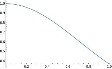
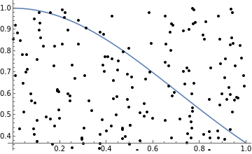
Clearly, the probability of any such a point being enclosed between the function and the y axis is equal to the ratio of the area enclosed by the function to the total area of the rectangle. Thus, the ratio of the number of points enclosed by the function to the total number of points, when multiplied by the area of the rectangle (which, in this case, is 1), gives an approximation to the value of the definite integral.

Approximating the Gaussian Integral

Higher-Dimensional Generalization

FURTHER EXPLORATIONS
Stratified Sampling
Importance Sampling
Mean Field Particle Methods
Umbrella Sampling (Computational Physics)
AUTHORSHIP INFORMATION
Jonathan Gorard
6/21/17