A brief description of the Metropolis–Hastings Monte Carlo Markov chain algorithm with examples.
June 24, 2017—Karthik Gangavarapu
Frequentist Approach to Inference
In a frequentist approach, data is random and the parameters are fixed. Inference is determined by finding parameters that maximize likelihood.
If we have some data and a model with parameters θ, then the Likelihood function, L(θ|), is defined in terms of the parameters of the probability density, P(|θ).
L(θ|)=P(|θ)
P(|θ) (often ln(P(|θ)), for ease of calculation) is maximized to infer the parameters θ for which the probability of attaining the data is highest.
For example, let's consider a biased coin. Let p be the probability of getting heads and (1-p) be the probability of getting tails.
Let's say we toss the coin 20 times, and we get 14 heads. A frequentist will calculate the maximum likelihood estimate of p as follows:
In[]:=
p=14/20//N
Out[]=
0.7
Formally, we can compute the maximum likelihood estimate using the binomial distribution as follows:
In[]:=
f[x_]:=Binomial[20,14]*x^14*((1-x)^6)
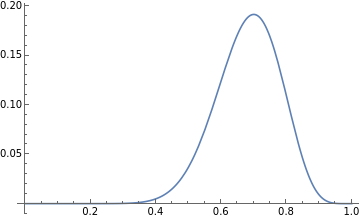
Let’s now plot this function:
In[]:=
Plot[f[y],{y,0,1}]
Out[]=
Now let’s find the maximum of this curve:
In[]:=
FindMaximum[f[y],{y,0,1}]
Out[]=
{0.191639,{y0.7}}
We see that the maxima occurs at y=0.7. This is equal to the the value p we calculated before.
The probability of getting n heads in n coin tosses will be p^n:
In[]:=
p^n
Out[]=
n
0.7
So the probability of getting two heads in two coin tosses is:
In[]:=
p^2
Out[]=
0.49
Bayesian Approach to Inference
In the Bayesian approach, the data is considered to be fixed, and the parameters θ are variable. Inference is performed by maximizing the posterior probability, f(θ|).
This posterior distribution is defined using the Bayes rule as:
The prior probability signifies the prior belief regarding the posterior distribution. The prior probability can have a large effect on the posterior probability, and thus care must be taken before picking one.
Let’s now see how Bayesian inference works in the same example we saw in the previous section. A biased coin is tossed 20 times, and we get heads 14 times. A Bayesian will treat the data to be fixed and the probability p to be a random variable with its own distribution.
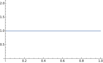
In the Bayes Rule, we see that the denominator f() is constant so, the posterior distribution, f(θ|) ∝ f(|θ) f(θ). A very convenient prior distribution to use for the binomial distribution is the beta distribution, which is also known as the conjugate prior of the binomial distribution. The uniform distribution is an instance of a beta distribution with the parameters a =1 and b = 1. Let's use a uniform prior distribution here, which basically means that we have no prior belief in the distribution of the posterior density function.
In[]:=
Plot[PDF[BetaDistribution[1,1],x],{x,0,1}]
Out[]=
We know the likelihood function, f(|θ) = f(|p):
In[]:=
Clear[f]f[x_]:=Binomial[20,14]*x^14*((1-x)^6)
Let’s now plot the function g(p|) = f(|p) f(p) ∝ f(p|):
The frequentist approach gives us a probability of 0.49, but the Bayesian approach gives us a probability of 0.47. This example illustrates the difference between the two inference methods.
The marginal probability, in real problems, is often hard to compute since it involves integration over all the parameters in the model. These integrals are often intractable. In order to ease this computation, Monte Carlo Markov chain (MCMC) techniques are used to sample the distribution without the need to compute such complex integrals.
Before getting into the algorithm, let's briefly go over what a Markov chain is in the next section.
What Is a Markov Chain?
A Markov chain is any stochastic process in which the next state of the system depends only on the current state. This property is formally called the Markov property.
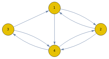
A Markov process is defined by a transition matrix that shows the probability of moving from one state to another. Shown below is a simple transition matrix for four states, "1", "2", "3", "4":
There are two types of Markov chains, discrete time and continuous time–based on, as the name suggests, whether the state of the system is defined in discrete time indices or in continuous time.
The Algorithm
To illustrate how the algorithm functions, it will be easiest to get an example first.
Let’s consider a normal distribution. In reality, since the distribution is in a closed-form expression, there would be no need to use the Metropolis–Hastings algorithm to sample it, but let’s use it as an example here.
Let's say we have data that is distributed in the form of a normal distribution. We want to sample this distribution.
Let's take a normal distribution with mean μ =1 and standard deviation σ=1 to be our posterior distribution:
For our prior probability distribution, let’s consider a uniform distribution, which is an uninformative prior i.e. it does not reinforce any prior belief we have in the distribution. If no knowledge of the final distribution is known, it is safer to use an uninformative prior like the uniform distribution or the Jeffreys prior.
Let’s pick a random starting parameter, θ1 for state 1:
Let’s now choose a parameter for state 2 by randomly sampling a proposal distribution. This is where the algorithm incorporates the Markov chain. This proposal distribution will be used to choose a new parameter to determine a new state for the system. Later, we will see how to set the probability of the system moving to the new state.
A usual proposal density that can be chosen is a normal distribution with the mean set as the parameter in the present state and a constant standard deviation.
Let’s choose a parameter θ2 for state 2.
Now let’s compute an acceptance probability to see if the system will transition from state 1 to state 2. This will be the transition probability of the Markov chain. If the posterior probability of the system at state 2 is higher than state 1, we definitely want to sample the parameter θ2 in state 2. On the other hand, if the posterior probability of the system in state 2 is lower than state 1, then we want to jump into state 2 with some probability.
So let's compute an acceptance probability α:
As you can see, marginal probability cancels out, and hence we can sample the entire distribution without computing the marginal probability (which, as discussed before, in more realistic problems can be computationally infeasible).
Note that probability cannot be greater than 1.
Let's restructure α such that the maximum value can only be 1.
This will be the probability with which we determine whether the MCMC will go to the new state.
To probabilistically make a move from one state to the next, we can generate a random number between 0 and 1. If the generated number is less than α, the system will move to the next state; otherwise, it will remain in the current state.
This step is repeated until we get a preset number of states. I’ve incorporated these steps into a function below:
Now let’s repeat the steps 1,000 times to get 1,000 samples from the posterior density.
Here’s a plot showing the prior distribution, posterior distribution and a normalized histogram of the sampled by the MCMC.
A common tool used to diagnose if the MCMC is running optimally is the trace plot. The trace plot is a plot of the current state of the system over time.
Let's now plot the trace plot of the distribution we just sampled.
We see from the trace plot that the MCMC is sampling parameters from all regions of the distribution. For convenience, let’s combine the function sampleWithMCMC and the commands used to plot into one function:
Let’s now run the combined function to repeat the sampling of the posterior distribution and plot the sampled distribution and trace plot:
This is how the Metropolis–Hastings algorithm is described formally.
Trace Plots
Sampling Multivariate Distributions
FURTHER EXPLORATIONS
Burn-in of MCMC Autocorrelation of Metropolis–Hastings MCMC Geweke’s Diagnostic for MCMC Techniques Other Proposal Distributions for Metropolis–Hastings MCMC Other MCMC Techniques—Gibbs Sampling, Slice Sampling, Adaptive Metropolis–Hastings