Measure of Center

The center of a distribution is a typical value that represents the group. We will discuss how the shape of the distribution might influence whether the mean is larger than, smaller than, or about the same as the median.
June 20, 2017—Jie Frye

Observations

Let’s take a look at the salaries from three university campuses.
View the data:
In[]:=
ResourceData["Sample Data: University Salaries"]
Out[]=
Department
FullTimeEmployment
Salary
Campus
IntercollegiateAthletics
1.
$
1.0525×
6
10
per year
A
Surgery
1.
$
650000.
per year
B
IntercollegiateAthletics
1.
$
600000.
per year
A
Surgery
1.
$
526250.
per year
B
Ophthalmology&VisualSci
1.
$
510625.
per year
B
Anesthesiology
1.
$
504000.
per year
B
Obstetrics&Gynecology
1.
$
485604.
per year
B
CancerBiology&Pharmacology
1.
$
482546.
per year
B
Surgery
1.
$
480000.
per year
B
Medicine
1.
$
462750.
per year
B
Surgery
1.
$
460000.
per year
B
Surgery
1.
$
456000.
per year
B
PresidentsOffice
1.
$
450000.
per year
A
AdministrationServices
1.
$
445740.
per year
B
Administration
1.
$
445740.
per year
B
Otolaryngology
1.
$
431109.
per year
B
Radiology
1.
$
430075.
per year
B
Medicine
0.99
$
422442.
per year
B
IntercollegiateAthletics
1.
$
405000.
per year
A
NeurologicalSurgery
1.
$
400000.
per year
B
showing 1–20 of 25438
We can see the salaries by department.
Organize the data by department:
In[]:=
data=GroupBy[ResourceData["Sample Data: University Salaries"],"Department"][All,All,"Salary"]
Out[]=
IntercollegiateAthletics
{
…
291
}
Surgery
{
…
112
}
Ophthalmology&VisualSci
{
…
90
}
Anesthesiology
{
…
58
}
Obstetrics&Gynecology
{
…
94
}
CancerBiology&Pharmacology
{
…
26
}
Medicine
{
…
342
}
PresidentsOffice
{
…
12
}
AdministrationServices
{
…
180
}
Administration
{
…
94
}
Otolaryngology
{
…
34
}
Radiology
{
…
37
}
NeurologicalSurgery
{
…
32
}
Psychiatry
{
…
339
}
OfcoftheChancellor
{
…
10
}
InternalMedicine
{
…
90
}
CtrforMagneticResonanceRsc
{
…
9
}
VPTechnology&EconomicDev
{
…
5
}
Pediatrics
{
…
208
}
CollegeofBusiness
{
…
48
}
showing 1–20 of 665
Let’s take a look at the distribution of the salaries of the surgery department, which is #2 in the data.
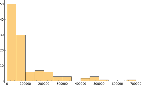
Make a histogram of 112 salaries in the surgery department in the data:
In[]:=
d=2;​​hist=Histogram[data[[d]]]
Out[]=
The shape of the salaries’ distribution of the surgery department is skew-right. The mean of the salaries of the surgery department is affected by the outlier $650,000 per year.
This finds the mean of the salaries:
In[]:=
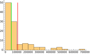
mean=QuantityMagnitude[Mean[data[[d]]]]
Out[]=
106748.
Is this a good estimate of the center of this distribution? Let’s take a look at the median.
This finds the median of the salaries:
In[]:=
median=QuantityMagnitude[Median[data[[d]]]]
Out[]=
51038.2
Which one is a better estimate of the center of this distribution?
Show the histogram, mean and median together:
In[]:=
Show[hist,ContourPlot[{xmean},{x,mean-1,mean+1},{y,0,50},ContourStyleRed,ColorFunctionAutomatic,FrameFalse,AxesTrue],ContourPlot[{xmedian},{x,median-1,median+1},{y,0,50},ContourStyleGreen,ColorFunctionAutomatic,FrameFalse,AxesTrue]]
Out[]=

Deciding Which Measurements to Use

Summary

Exercises

FURTHER EXPLORATIONS
Investigate the Wolfram Data Repository and explain your choice of measure of center for a dataset that you are interested in.

Initialization

AUTHORSHIP INFORMATION
Jie Frye
6/20/17