Lennard–Jones Potential

Or why perfume does not spread across your room in 0.02 seconds.
Mantas Pastolis

Derivation and Explanation of the Concept

It is known that when molecules are infinitely apart, they do not interact with each other.
Graphics[{​​Circle[{5,0},0.5],​​Circle[{-5,0},0.5],​​{Dashed,Line[{{-4.5,0},{4.5,0}}]}​​}]
However, as the molecules approach each other, they start interacting.
Graphics[​​Circle[{2,0},0.25],​​Circle[{-2,0},0.25],​​{Dashed,Line[{{-1.75,0},{1.75,0}}]},​​Arrow[{{-1.75,0},{-1,0}}],​​Arrow[{{1.75,0},{1,0}}],​​Arrowheads[{-0.04,0.04}],​​ Arrow[{{-2,-1},{2,-1}}],​​]
​
F
a
is the attractive force and r is the distance between the molecules/atoms.
When the molecules approach too closely to each other, they start to repel each other—repulsive forces dominate.
Graphics[{​​Circle[{0.25,0},0.25],​​Circle[{-0.25,0},0.25],​​Arrow[{{-0.5,0},{-1,0}}],​​Arrow[{{0.5,0},{1,0}}]​​}]
F
r
is the repulsive force between the molecules.
The natural question is: how do those two forces (attractive and repulsive) complement each other into one uniform system?
It turns out that attractive force can best be described by London dispersion forces: forces are induced by instantaneous electron density shift in atoms/molecules, which causes neutral atoms/molecules to have partially electronegative and electropositive sides.
This attractive energy can be described as:
U
a
(r)=-
3
2
α
1
α
2
I
1
I
2
I
1
+
I
2
·
1
6
r
The function can be simplified to:
U
a
(r)=-4ϵ
6
σ
r
Here, ϵ is the potential energy, required to infinitely separate two atoms from equilibrium distance
r
0
:
σ=
r
0
1/6
2
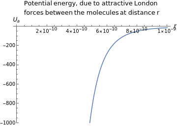
The attractive force is negligible at great distance, but becomes increasingly more significant as the atoms get closer.
Here is a typical shape of attractive energy potential with increasing distance (helium atoms are used for the example calculation):
Plot-4*11000*
6
258.*
-12
10
r
,{r,0,
-9
10
},​​ AxesLabelStyle["r",Medium,Black],​​ Style["
U
a
",Medium,Black]​​ ,​​ PlotLabelStyle["Potential energy, due to attractive London forces between the molecules at distance r",​​ FontSize13,​​ FontColorBlack​​ ],​​ PlotRange{0,-1000}​​ 
​
On the other hand, the repulsive force is described the by Pauli exclusion principle—no two electrons can occupy the same orbitals in an atom. If the two atoms get too close, their electrons start to share the orbitals. and therefore this repulsive force becomes highly dominant. It is described by:
U
r
(r)=-4ϵ
12
σ
r
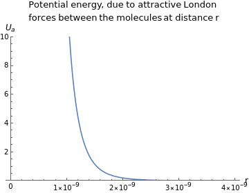
... which increases rapidly, as the atoms approach each other.
Here is the shape of the potential energy due to repulsive forces for helium atoms:
Plot4*11000*
6
258.*
-12
10
r
,{r,0,4*
-9
10
},​​ AxesLabelStyle["r",Medium,Black],​​ Style["
U
a
",Medium,Black]​​ ,​​ PlotLabelStyle["Potential energy, due to attractive London forces between the molecules at distance r",​​ FontSize13,​​ FontColorBlack​​ ],​​ PlotRange{0,10}​​ 
The total potential energy between the two molecules is:
U
total
(r)=-4ϵ
12
σ
r
-
6
σ
r

Therefore, the total function of potential energy between the two atoms/molecules can be viewed.
σ={258.*
-12
10
,342.*
-12
10
,427.*
-12
10
,527.*
-12
10
,412.*
-12
10
,297.*
-12
10
,406.*
-12
10
};(*sigmavaluesofthesubstances*)​​ϵ={11000,128000,536000,454000,368000,34000,236000};(*epsilonvalues*)​​textValues={"He","Ar","
Br
2
","
C
6
H
6
","
Cl
2
","
H
2
","Xe"};(*substancesused*)​​ManipulatePlot4ϵtype*
12
σ〚type〛
r
-
6
σ〚type〛
r
,{r,0,
-9
10
},(*creatingaplotforLennard-Jonespotentialfunction,whereσ〚type〛andϵ〚type〛arethe​​parameters,varyingwiththe"type"ofsubstance:*lookatthebottomofthecode*typevariesfrom1tothelengthofthelengthofσlist,​​andatthesametimethe"type"valuesfrom1to7areassignedtolookintheform"substance, σ value, ϵ value"*)​​ AxesLabelStyle["r",Medium,Black],​​ Style["
U
a
",Medium,Black]​​ ,​​ PlotLabelStyle["Overall potential energy between the molecules at distance r",​​ FontSize13,​​ FontColorBlack​​ ],​​ PlotRange{Automatic,{ϵ〚type〛/5,-ϵ〚type〛-2000}}​​ ,​​ {type,1,"Substance:"},Thread[​​ Range@Length@σRow/@​​ Riffle[#,", "]&/@​​ Transpose[{textValues,"(σ)"σ,"(ϵ)"ϵ}]​​]​​
However, the scale of interaction between the different molecules is not clear unless drawn within the same graph.

The Visualization of Interaction between the Particles

You can explore how two helium particles interact with each other in the following simulation. One particle can be adjusted at a fixed point, while the other interacts with the first one accordingly.
In this way, it is made sure that the particles will attract each other; however, the repulsive force prevents them from getting too close.
AUTHORSHIP INFORMATION
Mantas Pastolis