The Laplace transform is particularly useful in solving linear ordinary differential equations, such as those arising in analysis of electronic circuits.
June 23, 2017—Harish Chetty
What Is the Laplace Transform?
It is a method to solve differential equations. The idea of using Laplace transforms to solve differential equations is quite human and simple: it saves time and effort to do so, and, as you will see, reduces the problem of a differential equation to solving a simple algebraic equation.
But first let us become familiar with the Laplace transform itself. We now introduce a "prescription" for how to create a new function called F out of the old function f. The interesting part is that F will not depend on t anymore (as f does), but on an entirely new variable s.
You can say that we Laplace transform f from the t-space into F inside of the s-space.
The definition consists of two types of Laplace transforms. These are described in the following sections.
Definition of a Bilateral Laplace Transform
A two-sided (doubly infinite) Laplace transform for an input function given as i[t] is defined as:
This is the most common variety of Laplace transform, and it is what is usually meant by “the” Laplace transform. The unilateral Laplace transform L_t[f(t)](s) is implemented in the Wolfram Language as LaplaceTransform[function, t, s].
Generation of Laplace Transform for an Input Function
The Laplace transform is defined in the s complex domain. Here we’ll take an input function with regards to time (t) and try to obtain its Laplace transform in the complex form. This can be done with the following steps and with the use of FourierTransform.
Let’s take an Input function with respect to time into consideration.
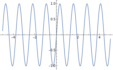
Plot a function as input data with respect to time. Here we take a Sin function as an input:
In[]:=
f[t_]:=Sin[5t]x=Plot[f[t],{t,-5,5}]
Out[]=
According to the definition mentioned, we multiply different exponential function as s where s is complex.
First we multiply the real part; here, that is
-at
e
where a is a real number.
Here we take three different values of a into consideration.
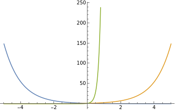
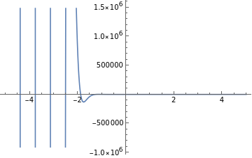
Plot different exponential functions as
-at
e
where t is time and a is a real number. We take three different cases where a=-1,1,7:
In[]:=
Plot[{E^-t,E^t,E^(7t)},{t,-5,5}]
Out[]=
Now, we multiply the input function with the real part of the exponential function, and get one step closer to achieving the fundamental definition of a Laplace transform.
Make a table by multiplying different function values of exponential a and plot their behavior using TableForm.
Here for each value of a, the graphical behavior is shown with it.
Now we can achieve the bilateral Laplace transform by applying FourierTransform to the system. But first...
What Is a Fourier Transform?
A Fourier transform converts a signal from the time domain (signal strength as a function of time) to the frequency domain (signal strength as a function of frequency).
Let's take an example into consideration. Take an input function with respect to time.
Create input data:
In[]:=
fourierInput=Exp[-t^2]Sin[t]
Out[]=
-
2
t
Sin[t]
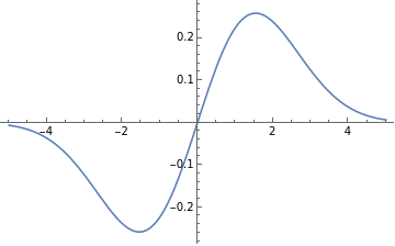
Now we take the Fourier transform of the input and, as per the definition, see if the output is in the frequency domain.
Apply the Fourier transform to the input function:
In[]:=
FourierTransform[fourierInput,t,frq]
Out[]=
(-1+Cosh[frq]+Sinh[frq])Cosh
1
4
2
(1+frq)
-Sinh
1
4
2
(1+frq)
2
2
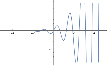
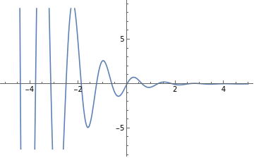
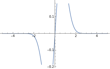
Here, the frq stands for the frequency. Let’s simplify to understand the equation better.
Apply Plot to the output for the frequency range for the imaginary part:
In[]:=
Plot[Im[fourierOutput],{frq,-5,5}]
Out[]=
FourierTransform gives the frequency in an imaginary plane, whereas the Laplace transform consists of both real and imaginary planes.
Thus, to obtain the imaginary part of the complex domain of the Laplace transform definition, we apply FourierTransform to the function.
Apply fourier to the real part; the output consists of a complex domain s:
For each value of a, a different value of the Laplace transform is obtained, as we observe in the above equations. The Laplace transform of the function is complex in nature, with a and ω. The obtained Laplace transform is bilateral, or a two-sided Laplace transform.
The following is a demonstration of the Wolfram Language built-in function LaplaceTransform.
Apply a unilateral Laplace transform to the initial input and examine the behavior.
The complex of the behavior is substituted with the variable s, where s consists of s = a + i ω, and thus the input function in the t domain is now transformed in the s domain.
Plot the Laplace transform in the s plane in 2D to see the behavior:
Now, let’s see the behavior in the complex plane with real and imaginary axes.
Use Plot3D to see the behavior in the complex domain:
The interesting part is that F will not depend on t anymore (as f does) but on an entirely new variable s. You can directly use f(t) and F[s]
Time vs. the S (Complex) Domain of the Laplace Transform
Laplace Transform vs. Fourier Transform
FURTHER EXPLORATIONS
Differential Equations Z Transform Region of Convergence Fourier Series Fourier Transform Poles and Zeroes