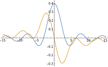
Thus, Fourier transforming a unit pulse gives sinc waves; however, we see that delaying the pulse gives rise to an imaginary component. If we think of t as time and ω as frequency, then the plots indicate that introducing a delay in the time domain results in a phase shift in the frequency domain.
The unit pulse is a fairly simple function. Calculating the Fourier transforms of more complex functions can be quite computationally intensive. However, Mathematica has built-in efficient Fourier transform capabilities.
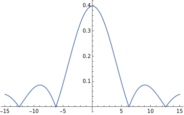
Here is a Fourier transform of a Gaussian modulated by a sinusoidal function:
In[]:=
ftGaussCos=FourierTransform[Cos[3t]Exp[-
2
t
],t,ω]
Out[]=
Cosh
1
4
2
(-3+ω)
2
2
+
Cosh
1
4
2
(3+ω)
2
2
-
Sinh
1
4
2
(-3+ω)
2
2
-
Sinh
1
4
2
(3+ω)
2
2
In[]:=
Plot[ftGaussCos,{ω,-7,7}]
Out[]=
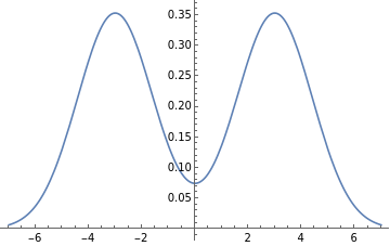
The Fourier transform shows which frequencies are present in a function of time. For example, the above plot shows that in our chosen Gaussian modulated by the sinusoidal function, ω = 3Hz is the dominant frequency.
Laplace Transform
Like the Fourier transform, the Laplace transform maps a real-valued function f(t) to a complex-valued function F(s). The difference, however, lies in the fact that unlike ω in the Fourier transform, s itself is a complex variable. So we can think of Laplace transforms as a way of selecting the complex frequencies present in the time-domain function f(t).
Here is a Laplace transform of sin(α t):
In[]:=
ltSin=Integrate[Exp[-st]Sin[αt],{t,0,Infinity}]
Out[]=
ConditionalExpression
α
2
s
+
2
α
,Abs[Im[α]]<Re[s]
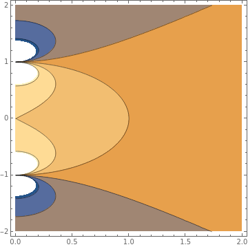
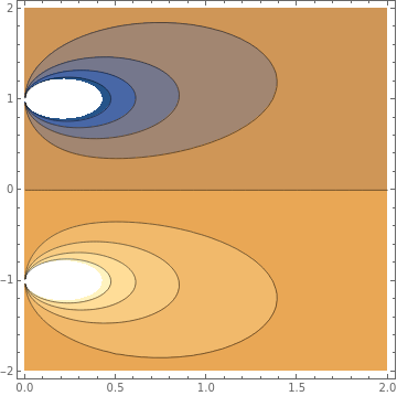
Let us try to visualize what this function of a complex variable looks like. For clarity, we will take α to be real; in fact, we will just put α = 1:
This is a bit different from the other three, yet closely related to them. Convolution is an integral transformation that takes in two functions of a real (or complex) variable and returns a third function of another variable (of the same type as the other variable).
Here is a convolution of the unit pulse and the inverse ramp functions:
We can do the same using the built-in convolution capabilities.
Here is a convolution of a Gaussian and a unit step function:
Inverse Transforms
These transforms would not be of much use if there were no transforms that were inverses of these. However, they do exist, at least in principle.
Inverse Fourier Transform
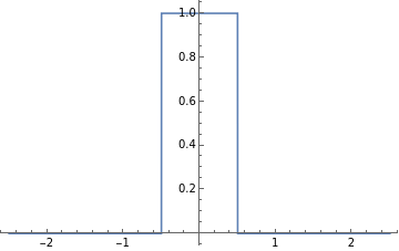
Here is an inverse Fourier transform of the sinc function. We should get a pulse as the answer:
It is indeed the unit pulse function.
Inverse Laplace Transform
Inverse Mellin Transform
The inverse Mellin transform is very similar in action to the inverse Laplace transform and plays an important role in number theory.
Let us see what happens to the Dirac delta when it undergoes the inverse Mellin transform: