Fourier Series

The Fourier series is a representation of a function as an infinite sum of sinusoids.
June 21, 2017—Michael Dobbs

The Fourier Series

History

Jean-Baptiste Joseph Fourier introduced the Fourier series as a way of solving the heat equation in a metal plate. In turn, he concluded that any arbitrary continuous function can be represented by a trigonometric series based on the set of
Sin(n·x)
and
Cos(n·x)
functions. In general, the techniques are quite useful when applied to differential equations involving eigensolutions that are sinusoids.

Motivation

Consider a function that does not have a closed-form integral formula (i.e. cannot be expressed without using numeric methods):
Plot said function,
Sin(
2
x
)
:
In[]:=
Plot[Sin[x^2],{x,-4,4}]
Out[]=
We attempt to the take the integral...
Integrate the function:
In[]:=
Integrate[Sin[x^2],x]
Out[]=
π
2
FresnelS
2
π
x
... and we can plot the function numerically.
Plot the integral formula:
In[]:=
Plot[%,{x,-4,4}]
Out[]=
However, there does not exist a closed-form solution to such an integral equation.

Theory

We can define a series of sinusoids that converge to the original function, with the correct constants.
Find the first coefficient in the Fourier series:
In[]:=
FourierCoefficient[Sin[x^2],x,1]
Out[]=
-
1
8
π
1/4
(-1)
-

4


2

Erf
1
2
1/4
(-1)
(1-2π)-Erf
1
2
1/4
(-1)
(1+2π)-Erfi
1
2
1/4
(-1)
(-1-2π)+Erfi
1
2
1/4
(-1)
(-1+2π)
Express it numerically:
In[]:=
N[%]
Out[]=
0.096227-1.38778×
-17
10

Create a list of the first three coefficients in the series:
In[]:=
Table[FourierCoefficient[Sin[x^2],x,i],{i,1,3}]
Out[]=
-
1
8
π
1/4
(-1)
-

4


2

Erf
1
2
1/4
(-1)
(1-2π)-Erf
1
2
1/4
(-1)
(1+2π)-Erfi
1
2
1/4
(-1)
(-1-2π)+Erfi
1
2
1/4
(-1)
(-1+2π),-
1
8
π
1/4
(-1)
-


2

Erf
1/4
(-1)
(1-π)-Erf
1/4
(-1)
(1+π)+Erfi
1/4
(-1)
(-1+π)+Erfi
1/4
(-1)
(1+π),-
1
8
π
1/4
(-1)
-
9
4

9
2

Erf
1
2
1/4
(-1)
(3-2π)-Erf
1
2
1/4
(-1)
(3+2π)-Erfi
1
2
1/4
(-1)
(-3-2π)+Erfi
1
2
1/4
(-1)
(-3+2π)
In[]:=
N[%]
Out[]=
{0.096227-1.38778×
-17
10
,-0.00837573+6.48353×
-17
10
,-0.340173+2.77556×
-17
10
}
We attach these constants to the corresponding functions and obtain an approximation.
Create the first-order Fourier series of the function:
In[]:=
FourierSeries[Sin[x^2],x,1]
Out[]=
-
1
8
π
1/4
(-1)
-

4
+x


2

Erf
1
2
1/4
(-1)
(1-2π)-Erf
1
2
1/4
(-1)
(1+2π)-Erfi
1
2
1/4
(-1)
(-1-2π)+Erfi
1
2
1/4
(-1)
(-1+2π)-
1
8
π
1/4
(-1)
-

4
-x


2

Erf
1
2
1/4
(-1)
(1-2π)-Erf
1
2
1/4
(-1)
(1+2π)-Erfi
1
2
1/4
(-1)
(1-2π)+Erfi
1
2
1/4
(-1)
(1+2π)+
FresnelS[
2π
]
2π
Create the third-order Fourier series of the function:
In[]:=
fourierSeries3=FourierSeries[Sin[x^2],x,3]//N
Out[]=
0.245943+(0.0932356+0.0238069)
(0.-0.25)-(0.+1.)x
2.71828
+(0.0932356+0.0238069)
(0.-0.25)+(0.+1.)x
2.71828
-(0.00452542+0.00704793)
(0.-1.)-(0.+2.)x
2.71828
-(0.00452542+0.00704793)
(0.-1.)+(0.+2.)x
2.71828
+(0.213688-0.264679)
(0.-2.25)-(0.+3.)x
2.71828
+(0.213688-0.264679)
(0.-2.25)+(0.+3.)x
2.71828
We can plot said function with
Sin(
2
x
)
to compare.
Plot Sin(
2
x
) and our Fourier series approximation on the same graph:
In[]:=
Plot[{Sin[x^2],fourierSeries3},{x,-4,4},PlotLegends"Expressions"]
Out[]=
sin(
2
x
)
fourierSeries3

Mathematical Exploration

While we can see that the functions do not overlap exactly, we will explore the convergence of the series.
Create the first-order Fourier series approximation:
In[]:=
fourierSeries1=N[FourierSeries[Sin[x^2],x,1]];
Plot it:
In[]:=
Plot[{Sin[x^2],fourierSeries1},{x,-4,4},PlotLegends"Expressions"]
Out[]=
sin(
2
x
)
fourierSeries1
Create the fourth-order Fourier series approximation:
In[]:=
fourierSeries4=N[FourierSeries[Sin[x^2],x,4]];
Plot it:
In[]:=
Plot[{Sin[x^2],fourierSeries4},{x,-4,4},PlotLegends"Expressions"]
Out[]=
sin(
2
x
)
fourierSeries4
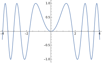
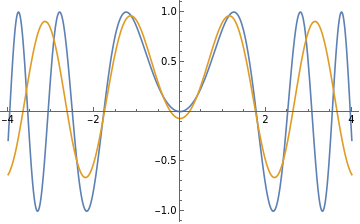
Create the seventh-order Fourier series approximation:
Plot it:

Application: Numerical Analysis

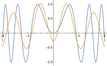
We can then compare the numerical integral to the integral of the Fourier series (of which all the terms are integrable).
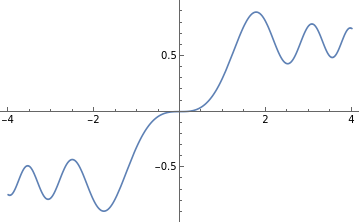
Compute a list of differences between the integrals as the order of the series increases and plot:
We can see that the difference is tending toward 0. Thus, taking the integral of the Fourier series of a function is one way to approximate the area under a curve.

Another Application: Solving Differential Equations

First find the Fourier series of the right-hand side of the equation. We show the first few terms here:
To begin, we compute the second derivative on the left-hand side of the equation for each term:
We then solve for the unknown coefficients, after generalizing the coefficients on the right-hand side. For the even terms:
For the odd terms:
FURTHER EXPLORATIONS
Explore the Taylor Series Expansion of a Function
Explore Other Sets of Basis Functions That Can Approximate a Function
AUTHORSHIP INFORMATION
Michael Dobbs
6/21/17