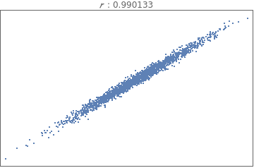
Correlation is a measure of the strength of a linear relationship between two numerical variables.
June 21, 2017—Silvani Vejar
Why Do We Care About Correlation?
Correlation is important in statistics because it allows us to quantify the relationship between quantities. For example, you probably have wondered if there’s a relationship between things like the amount of calories you consume and your weight, number of fast-food restaurants in a neighborhood and obesity rates, income and mortality rates, etc. The strength of a linear relationship between quantities like these ones is measured using the linear correlation coefficient. When we say two variables are correlated, we are saying that the variables seem to have a strong relationship between each other, but be careful—correlation does not imply causation.
The correlation coefficient
measures the strength of a linear relationship between two paired numerical variables, and it describes the direction (positive or negative) and strength of a relationship between two variables (how well data fits a straight-line pattern).
With the help of the Wolfram Language and data from the Wolfram Data Repository, we will be able to do an overview on calculating and interpreting the correlation coefficient.
Correlation Coefficient Properties
only measures the strength of a linear relationship. There may be nonlinear relationships.
is always between
–1
and 1 inclusive;
–1
means a perfect negative linear correlation and
+1
means a perfect positive linear correlation.
has the same sign as the slope of the regression (best-fit) line.
does not change if the independent (
x
) and dependent (
y
) variables are interchanged.
does not change if the scale on either variable is changed. You may multiply, divide, add or subtract a value to/from all the
x
values or
y
values without changing the value of
.
has a Student's
t
-distribution.
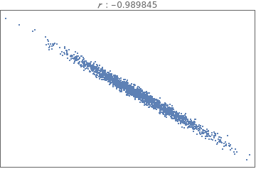
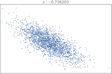
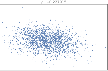
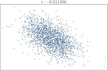
Comparing and Interpreting Linear-Strength Relationships from Scatter Plots
ToExpression::sntxi: Incomplete expression; more input is needed .
In[]:=
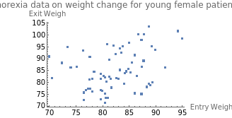
The data below shows the before and after weights of young women undergoing anorexia treatment. When you look at the data, what kind of questions might you ask?
Obtain data from the Data Repository: before and after weights of young women undergoing anorexia treatment:
By simply looking at data in a table, it can be difficult to observe whether or not there is a linear relationship between the entry weights and exit weights of the young female patients. A scatter diagram can help us to visualize the distribution of the data.
By looking at the scatter plot, would you say there is a correlation between the entry and exit weights of the young female patients? The data is widely scattered, and with a visual inspection we can observe that there doesn’t seem to be a strong correlation between these two variables. But to be sure, let’s calculate the value of
We found the value of the linear correlation coefficient,
=0.332406
,but what does it mean? To interpret its meaning, we can use our knowledge on hypothesis tests and p-values (which indicate that there is a weak linear relationship between the entry and exit weights, and we can conclude that the weights of the patients are random and there is no evidence to support that the anorexia treatments are effective).
In cases where we find a strong linear correlation, we can proceed to a hypothesis test and find the line’s best fit.
To interpret
,we refer to the computed p-value. If it is less than or equal to the significance level, we conclude there is a linear correlation.
Hypothesis Test Using the
p
-Value from a
t
-Test
Using the previous example, we can conduct a formal hypothesis test of the claim that there is linear correlation between the entry and exit weights.
To claim that there is linear correlation implies that the linear correlation coefficient is not zero:
H
o
:ρ=0
: There is no linear correlation
H
1
:ρ≠0
: There is linear correlation
(*In cases where we find a strong linear correlation, we can proceed a hypothesis test and find the line best-fit.*)
Plot the data points and the regression line:
In[]:=
model["ParameterConfidenceIntervalTable"]
Out[]=
Estimate
StandardError
ConfidenceInterval
1
42.7006
14.4311
{13.9186,71.4826}
x
0.51538
0.174777
{0.166799,0.863962}
Coefficient of Variation
2
—Explained Variation
In cases where we conclude there is a linear correlation between the two variables, we can find a linear equation that expresses y in terms of
x
(linear regression). The value of
2
is the proportion of the variation in
y
that is explained by the linear relationship between the two variables.
In[]:=
model["RSquared"]
Out[]=
0.110494
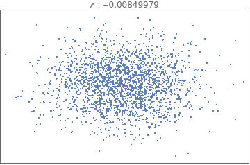
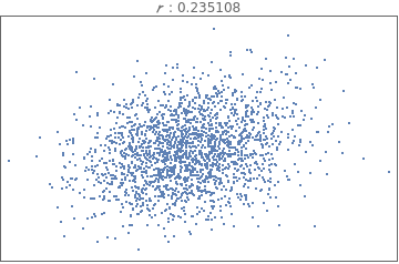
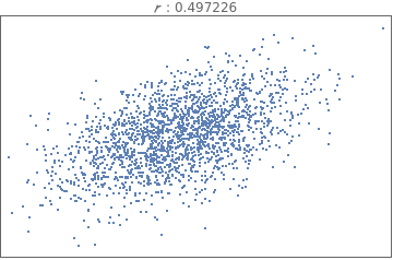
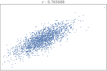
What does it mean to say there is a positively or negatively linear relationship between two variables?
Practice Questions
Using the Data Repository, choose a set of data and create your own notebook to do the following:
1
.
Load data
2
.
Create a scatter plot
3
.
Based on the scatter plot, provide an estimation for the value of the correlation coefficient between the two variables and explain your answer.