Differential Drive

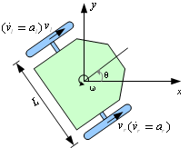
Differential drive is one of the configurations for robot mobility. It consists of two driven wheels on each side of the robot, and maybe some free wheels for stability. Each of the driven wheels has encoders that are able to count the revolutions in terms of angles or that are derived to speed with simple geometric equations.
Santiago Sánchez Vasquez

Import Images

Import["https://www.cse.unr.edu/robotics/tc-apc/sites/cse.unr.edu.robotics.tc-apc/files/differenticalfigure.png"]
Column[{Import["http://hades.mech.northwestern.edu/images/2/22/Encoder_diagram.png"],Import["http://img.directindustry.com/images_di/photo-g/5789-2409187.jpg"]}]

ConversionFactor

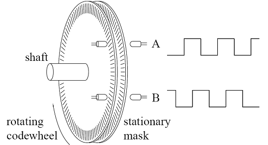
The first task is to convert the pulses of the encoder into a linear displacement. This can be done with the following equation, which will give us a result of a factor that we’ll call
f
.
f[d_,N_]:=
d*π
N
Where
d=diameter
of the wheel and
N=number
of pulses.
Set up your own specifications.
F=Manipulate[N[Table[f[Diameter,NumPulses],1]],{Diameter,1,40,1,Menu},{NumPulses,1,200,1,Menu}]
​
Diameter
40
NumPulses
300
{f[40.,300.]}

LinearVelocity

The linear velocity of the robot is calculated with the following equation.
Vlin[Vr_,Vl_,F_]:=
Vr+Vl
2
*F
You can change the linear velocity of your robot by setting the next parameters.
​​Vl=Manipulate[Table[Vlin[Vright,Vleft,F],1],{Vright,1,20,1},{Vleft,1,20},{F,0,10,0.0001,Menu}]
​
Vright
Vleft
F
0
{Vlin[1,1,0]}
​

Angular Velocity

CurrentPosition

Future Work

The following steps, which are not within the scope of this document, include the implementation of a PID controller with a constant linear velocity and setting a goal at a desired theta, which is taken from the following equation.
θdes=ArcTan[Sin[Ygoal-Y]/Cos[Xgoal-X]]​​
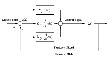
Now theta is the desired setpoint for the PID controller, and it is subtracted from the current theta, generating the error e(t) for the controller.
Import["https://qph.ec.quoracdn.net/main-qimg-f80e2346eca7905cdc90e38450483be6"]