Seriously?! You have never heard about deep convolution neural networks, have you? Deep convolution neural networks are state-of-the-art algorithms in many computer vision problems, such as image classification or detection.
Ooww, come on! State-of-the-art algorithm? What do you mean by this?
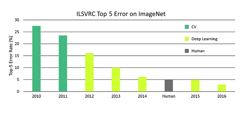
Have you heard about ImageNet Large Scale Visual Recognition Challenge (ILSVRC)? Probably not. The goal of this competition is to predict one of the thousands of classes used to describe images.
Please take a look at the competition results over time.
As you can see, since 2012 there has been a huge improvement of the detection algorithm's performance.
Hmmm. OK, fine! So you mentioned the deep neural network. How does it work?
Generally, this model has a formulation that can map your input
x
all the way to the target objective
y
via a series of hierarchically stacked (this is where the "deep" comes from) operations.
Those operations are typically linear operations/projections (
W
i
), followed by non-linearities (
f
i
), like so:
y=
f
N
(…
f
2
(
f
1
(
T
x
W
1
)
W
2
)
…W
N
)
(
1
)
One of the most traditional and easiest-to-understand deep learning architectures is known as a multilayer perceptron (MLP). In that kind of network, every element of a previous layer is connected to every element of the next layer. It looks like this:
Ohhh! I just realized something. You said, “Every element of a previous layer is connected to every element of the next layer.”
So let us assume our input is 10D, and we have a first layer of 20 hidden units. So in this very basic example,
W
1
∈
10x20
R
, and that means a lots of weights to be tuned.
How about the images? The simple image is a NxM matrix, so your input is
N·M
-dimensional, e.g. a small image (64x64 pixels) tends to generate inputs of 4096D! Deal with it!
Yes! You are definitely right. The MLP model is not designed to work with images. Nevertheless, it is very useful when you are working on categorical data and your input is low-dimensional.
OK, fine. So how about the images? Do you know any other deep learning architectures designed for analyzing images?
“Patience you must have, my young Padawan.” Before we move on to convolution networks, I would like to explain to you the idea of convolution operation. Let us start with the basics. What is convolution?
Convolution is the process of adding each element of the image to its local neighbors, weighted by a kernel. This is related to a form of mathematical convolution.
For example, the element at coordinates {2,2} (that is, the central element) of the resulting image would be calculated in the following way:
I suppose you noticed that this operation's time complexity for NxM images and kxk kernel is
O(MNkk)
.
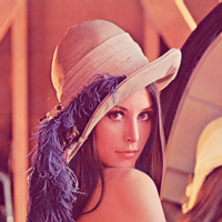
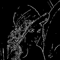
Now, I would like to show you a couple examples of different kernels.
But first I need to import an exemplary image. I will take the image of Lena. It is the name given to a standard test image widely used in the field of image processing since 1973.
Wow Dude! That was awesome! But why are you talking about this? You were supposed to present neural networks!
As you see, the convolution filters are a very powerful tool. But we need to figure out the kernel size and parameters. This is not a trivial task. It would be very nice if we found a way to somehow learn the weights. Here come deep convolution neural networks. An exemplary architecture of that kind of network is presented here.
On demand, I can add a short introduction to pooling and nonlinearity layers.
Please show me some examples. How do I build and train that kind of network?
Yes, sure. For the purposes of this example, I will use the MNIST dataset. It is a large database of handwritten digits.
The MNIST database contains 60,000 training images and 10,000 testing images.
We have a dataset. That is good. Now let us construct a shallow convolution neural network. Our network contains only two hidden convolution layers. You will see that this architecture allows us to obtain great results.
Now it is time to train our network.
Here comes my question. How can I preserve learning curve plots? How can I visualize gradient flow?
Now I want to check the network's performance with a first, basic test. Let's take a look at the first 100 test events.
The above test is very naive. We are not able to look at each of the test examples. We need to do something a little bit smarter. We can base our judgment on the classifier performance measurement metric’s accuracy. Accuracy is a description of systematic errors—a measure of statistical bias—as these cause a difference between a result and a “true” value. In other words, it gives you a ratio of a correctly classified example to all of the test examples. So the best possible value, a perfect classification, is 1.
What does this result mean?
It basically tells you that this classifier returns a correct prediction roughly 99% of the time. Another way of looking at the classifier performance is a so-called confusion matrix. Each column of the matrix represents the instances in a predicted class, while each row represents the instances in an actual class. The name stems from the fact that it makes it easy to see if the system is confusing two classes (i.e. commonly mislabeling one as another).