This topic explains the logic behind the backpropagation functionality in neural networks.
June 23, 2017—Tetyana Loskutova
Preparatory Reading
Perceptrons Sigmoid (logistic) function
The History of the Backpropagation Algorithm
Backpropagation is a training algorithm for neural networks that allows the training to progress through multiple layers. The basic idea behind neural network computing is the adjustment of neuron weights based on the difference between the result produced by the neuron and the required result. However, the required result is known only for the output layer, which creates a problem when adjusting the weights of hidden layers. For some time, this problem stalled the development of the machine learning field. The breakthrough came with the formulation of the backpropagation algorithm. The basic idea of backpropagation is: 1) to use calculus to assign some of the blame for any training set mistake in the output layer to each neuron in the previous hidden layer; and 2) to further split up the blame for the previous hidden layers (if such blame exists) until the input layer is reached. This method of splitting and assigning the blame is essentially backpropagation of the error.
Backpropagation Example
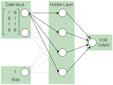
As is clear from the history, backpropagation requires a network with at least one hidden layer. In this example, a three-layer network will be used for a demonstration of the algorithm.
Backpropagating neural networks learn by example—that is, they require a set of inputs and associated outputs.
Initialize an input matrix:
In[]:=
(x={{0,0,1},{0,1,1},{1,0,1},{1,1,1}});
Initialize an output matrix:
In[]:=
(y={{0},{1},{1},{0}});
In[]:=
Grid[{x//MatrixForm,y//MatrixForm}]
Out[]=
Grid
0
0
1
0
1
1
1
0
1
1
1
1
,
0
1
1
0
It is easy to see that the problem is basically a logical XOR operation and the third row in the input does not contribute toward the output; however, it makes the problem appear harder. The third input in this case is sometimes called “bias”.
To demonstrate backpropagation, the network should first complete a first feedforward propagation and estimate the output.
Since the weights are initiated randomly, it is a good practice to reset the random generator:
In[]:=
SeedRandom[];
Initialize weights that will be used to generate the inputs to the hidden layer. weights21 is the weight between the second (hidden) and first (input) layers. weights21 is a 3x4 matrix that connects each of the three input neurons to the four hidden neurons:
In[]:=
(weights21=RandomReal[{-1,1},{3,4}]);
weights32 connects the four hidden neurons to the one output neuron; thus, they are shaped as a 4x1 matrix:
In[]:=
(weights32=RandomReal[{-1,1},{4,1}]);
The basic formula for the feedforward pass contains two steps:
1
.
Find the input to the next layer’s neuron as a sum of the outputs of the previous layer’s neurons multiplied by weights, in other words a dot-product of the previous layer outputs and weights;
2
.
Apply the activation function. In this example, a logistic sigmoid function is used. Other activation functions also exist, such as Tanh, ArcTanh, ReLU, etc.
The input layer is equal to the input matrix:
In[]:=
inputs=x;
Compute the hidden layer:
In[]:=
hidden=LogisticSigmoid[inputs.weights21];
Compute the output layer. This is the first and very inaccurate approximation of the output:
In[]:=
outputs=LogisticSigmoid[hidden.weights32]
Out[]=
{{0.554772},{0.572816},{0.522067},{0.538946}}
Backpropagation
The first step in backpropagation is to calculate the errors:
In[]:=
outputsError=y-outputs
Out[]=
{{-0.554772},{0.427184},{0.477933},{-0.538946}}
Logistic Sigmoid
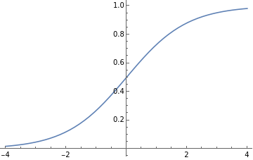
The next step demonstrates the magic of backpropagation and explains the need for the activation function, which is plotted below:
In[]:=
Plot[LogisticSigmoid[x],{x,-4,4}]
Out[]=
In the forward propagation pass, the values of the sigmoid function are applied to the sum of the inputs to the neuron layers. The plot above shows that higher absolute values of
x
are characterized by a sufficiently confident value of y close to 1 or 0. However, the values near
x=0
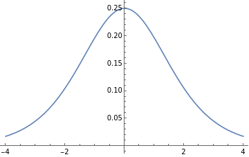
are close to 0.5 and do not allow a confident prediction. Therefore, these not-confident values must be updated by a higher value. To make such an update, the derivative of the sigmoid function is used (pictured below). The derivative produces higher values of the update coefficient in the area near
x=0
, while higher absolute values of
x
are associated with very small update coefficients.
Here are the values of the derivative of the sigmoid function:
In[]:=
Plot[LogisticSigmoid'[x],{x,-4,4}]
Out[]=
Backpropagating Errors
Find the update value for the weights between the output and the hidden layers using the derivative of the sigmoid to heavily update the non-confident predictions:
For the hidden layer, the errors cannot be calculated because there is no information about what the values of the neurons in this layer should be. Instead, these errors are estimated based on the values of the required update between the output and the hidden layer:
In[]:=
hiddenError=outputsDelta.Transpose[weights32];
The update for the weights in the hidden layer is also estimated using the derivative of the sigmoid function:
In[]:=
hiddenDelta=hiddenError*LogisticSigmoid'[hidden];
Finally, the weights are updated based on the values of the previous layer and the update values:
The recalculated weights are used again to calculate the next forward propagation step. The process is repeated until the error in the output layer is sufficiently small or the allowed number of iterations has been reached (the latter may be necessary for the problems that do not arrive at a high-precision solution).
Working Example
Below, all the code from the previous section is put together in a training cycle, which runs for 10,000 iterations: