The artificial neuron is the basic building block of artificial, convolutional and other popular neural networks, and forms the basis of most of modern deep learning.
June 23, 2017—Rohan Saxena
Modeling the Artificial Neuron
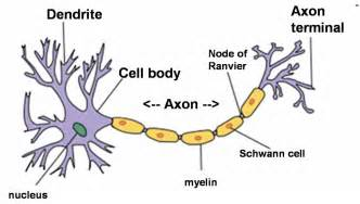
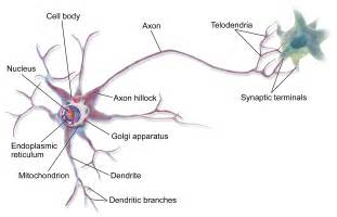
Historically, the artificial neuron is supposed to have developed from the biological neuron. Let’s try to visualize that.
Pull up a couple of images of a biological neuron.
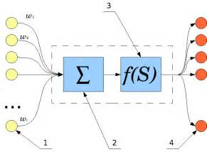
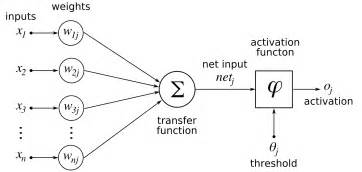
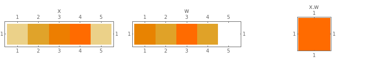
In the analogy of the biological neuron, the value of x.w tells us how intense the inputs collected from the dendrites are (by getting scaled up by the weight vector w) once they have entered the neuron. The higher the value, the more intense the input.
Axon
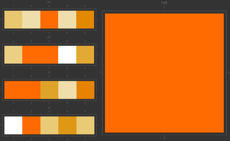
Looking back at the picture of the artificial neuron, we see that this part sums up a lot of vector products.
The value of the activation (output) of the neuron tells us how intense a signal the neuron is sending to the subsequent neurons in the network.
Axon Terminal
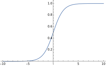
This part uses something called an activation function. An activation function introduces nonlinearity into the values of the neuron. Let’s look at some activation functions.
Plot the sigmoid function.
Plot[LogisticSigmoid[x],{x,-10,10}]
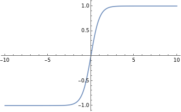
Plot the tanh function.
Plot[Tanh[x],{x,-10,10}]
The tanh function seems to be steeper than sigmoid, and hence is closer to the discontinuous function plotted below.
The above functions are basically differentiable approximations for the following function.
The above function is useful for binary classification (0 being one class, 1 being another). We use the above functions instead because they are differentiable and allow us to use our good friend calculus.
We’ll look at some other popular activation functions.
Applications
FURTHER EXPLORATIONS
Backpropagation Training a neural network Recurrent neural network, long short-term memory (LSTM)